The Architecture of Memory and the Mathematical Scramble: A Deep Dive into Google TurboQuant
The modern landscape of large language model (LLM) deployment is characterized not by the raw speed of mathematical calculation, but by the physical constraints of memory architecture and the persistent “memory tax” of high-dimensional data.
In the world of backend engineering and software architecture, the most elegant algorithms are often those that solve fundamental bottlenecks by returning to first principles—understanding exactly how bits are moved, where they are stored, and what the cost of retrieval is. Google Research’s introduction of TurboQuant (TQ) represents such a shift, providing a mathematical blueprint to dismantle the primary bottleneck in AI inference: the Key-Value (KV) cache. To understand TurboQuant, one must first dissect the inner workings of the modern AI “working memory” and why traditional compression techniques have historically failed to deliver efficiency without sacrificing quality.
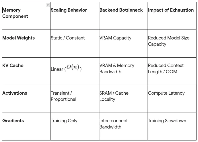
The Fundamental Bottleneck: Dissecting the KV Cache
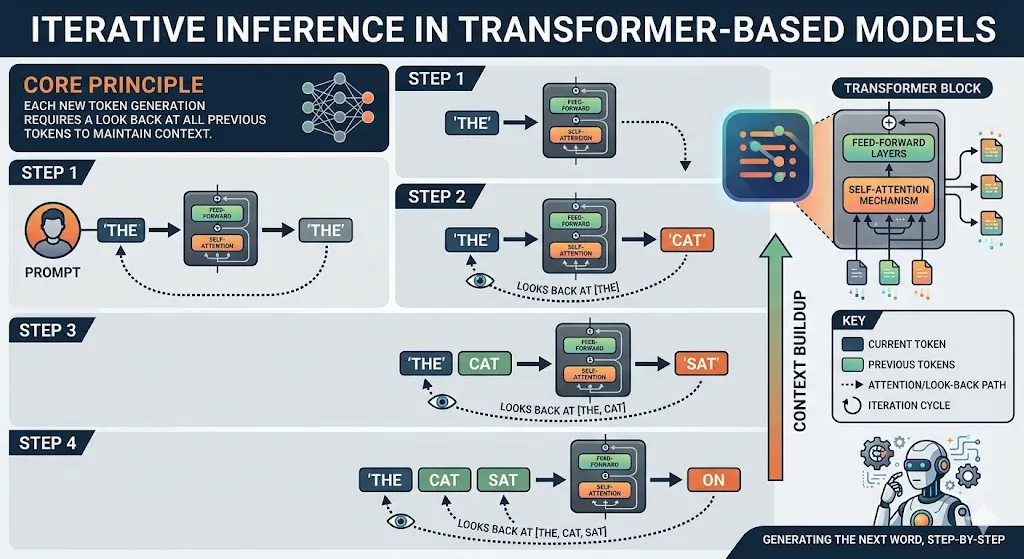
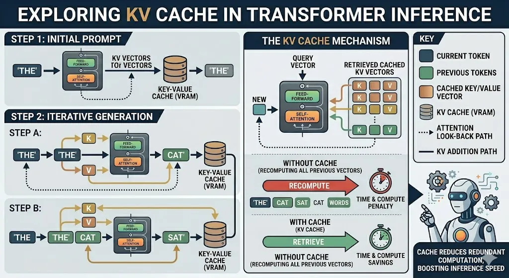
In the architecture of a transformer-based model, the inference process is inherently iterative. Each time a model generates a new token, it must look back at all previous tokens to maintain context.
This look-back is facilitated by the KV cache, which stores the mathematical representations (keys and values) of every token processed in a session. Conceptually, the KV cache acts as a high-speed “digital cheat sheet,” allowing the computer to retrieve information instantly without recomputing the entire history of a conversation for every new word generated.
However, this architecture introduces a linear scaling problem. As the context window grows—whether in a long chatbot conversation, a narrative scene generation, or a complex video transformer sequence—the memory required to store these KV pairs expands proportionally. This growth places immense pressure on the GPU’s Video Random Access Memory (VRAM), a resource that is significantly more scarce and expensive than standard system RAM. When the VRAM is exhausted, the system experiences a “memory wall,” leading to slowdowns, higher latency, or total system crashes.
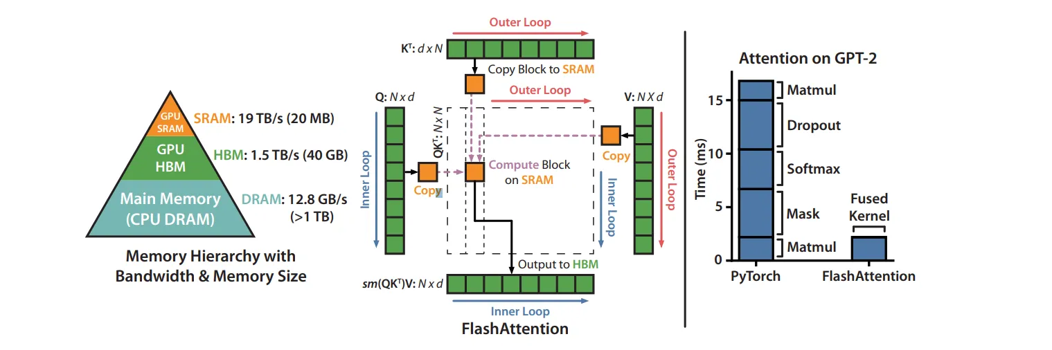
The beauty of the problem lies in the realization that inference is rarely compute-bound; it is almost always I/O-bound. The time taken to move data from High-Bandwidth Memory (HBM) to the processor’s Static RAM (SRAM) is the real bottleneck.
Consequently, reducing the size of the data moved is the most effective way to speed up the entire pipeline.
The Efficiency Tax: Why Traditional Quantization Fails
Quantization is the process of mapping a large set of continuous values (like high-precision 16-bit or 32-bit decimals) to a smaller, discrete set of symbols (like 4-bit or 8-bit integers). While this should theoretically reduce memory usage by 4x or 8x, the implementation of traditional vector quantization (VQ) carries a “leaky” quality that results in an “efficiency tax”.
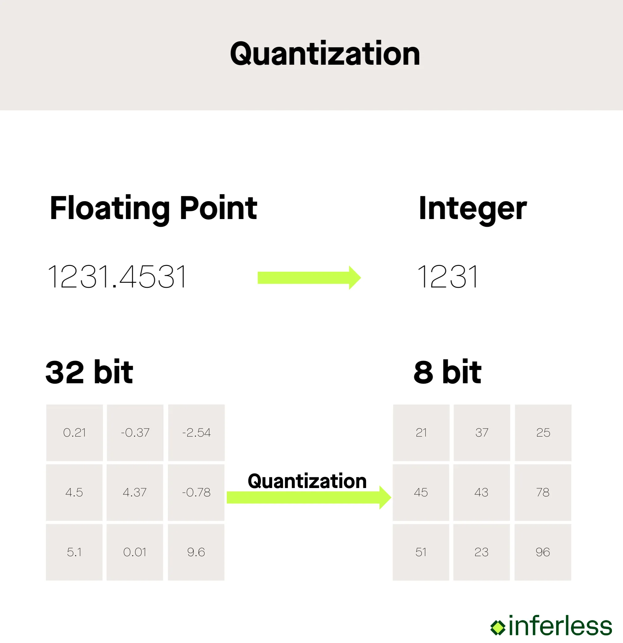
The genius of this tax lies in the “quantization constants.” When a system compresses data, it must store meta-data—normalization values and scale factors—to tell the model how to decompress the data accurately. In many aggressive 4-bit schemes, these constants add an extra 1 to 2 bits of overhead per value. This means a “4-bit” quantizer might actually use 6 bits of memory per channel, significantly diminishing the practical gains.
Furthermore, traditional Vector Quantization (VQ) often relies on data-dependent calibration or “training” (such as k-means clustering), which makes it difficult to use in real-time, online inference where the data distribution might shift unexpectedly.
If the quantization is too aggressive without proper mathematical grounding, the model begins to suffer from “quantization error,” which accumulates and manifests as hallucinations or a loss of semantic coherence. This is where TurboQuant enters the picture, aiming to provide “quality neutrality”—extreme compression (3 bits or fewer) with zero measurable loss in accuracy.
Under the Hood: The TurboQuant Architecture
TurboQuant is not a single trick but a sophisticated, two-stage mathematical pipeline designed to operate near the theoretical lower bounds of distortion. It achieves its results—a 6x reduction in memory and up to an 8x speedup—by decomposing the vector quantization problem into two distinct steps:
- high-quality geometric compression (PolarQuant)
- unbiased error correction (QJL).
First Principles: The Random Rotation (Whitening)
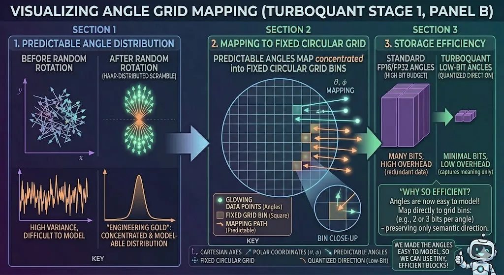
Before any compression occurs, TurboQuant applies a random rotation to the input vectors. To understand the brilliance of this, consider a high-dimensional dataset as a messy, unstructured spreadsheet with values scattered all over the place. Some columns have massive values; others are tiny. Compressing this “raw” data is difficult because the quantizer must account for these wild variations.
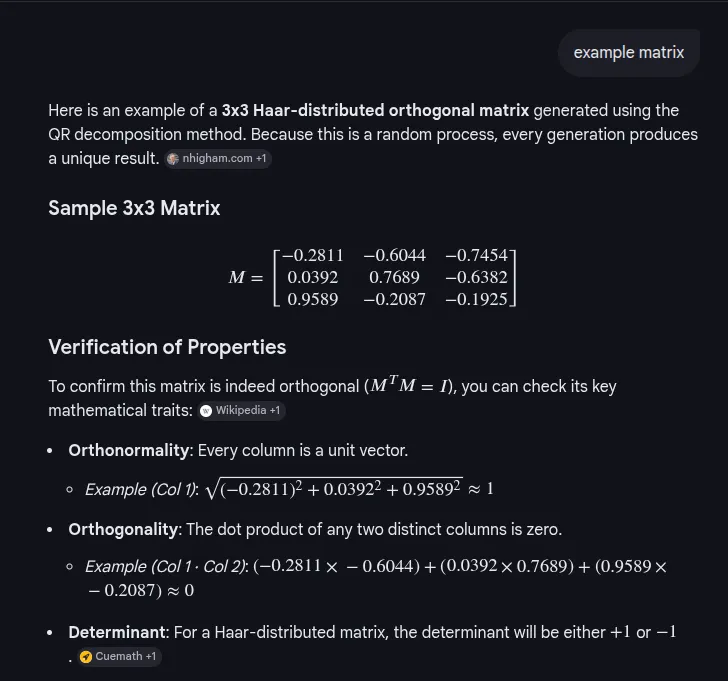
By applying a Haar-distributed orthogonal matrix—essentially a mathematical “scramble”—TurboQuant projects the vectors into a new coordinate system. This process, known as whitening, spreads the energy of the data uniformly across all dimensions. In this rotated space, the coordinates follow a concentrated Beta distribution. This makes the data’s geometry predictable and uniform, allowing the system to use standard scalar quantizers on each part of the vector individually.
They say it’s a Haar-distributed orthogonal matrix. Forget “Haar.” Forget “matrix.” What does it do? It is a rotation. Think of it like taking a photo and spinning it. You aren’t changing the objects in the photo, you are changing your perspective on them. That’s what a “unitary transform” is. It is a coordinate shift that preserves length. The distance between the points doesn’t change. But the values on the axis do change.
And they are spinning it in a very specific, random way. That’s the “scramble.”
Why do this? Look what happens to the energy distribution. The text says it “spreads the energy of the data uniformly across all dimensions.” This is the key. Remember that messy distribution where some dimensions were empty and some were massive? After this rotation, that variability is gone. Every single dimension gets an equal portion of the total “information” or “energy.” They are all homogenized.
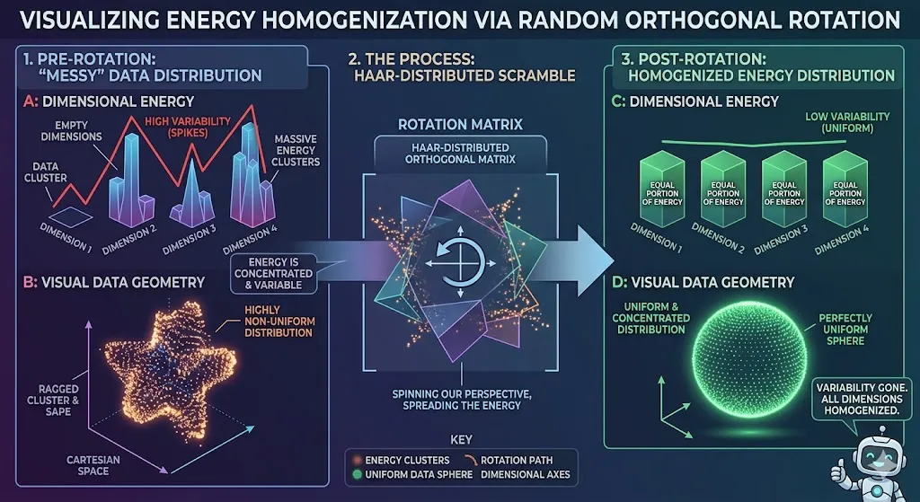
So, picture this: your data went from a spiky, clustered, unpredictable distribution to a perfectly uniform, predictable sphere, or “hypersphere” in higher dimensions. It’s smooth. It’s symmetric. It looks exactly the same from every angle.
Now, we are in a completely different world! This rotated space has beautiful properties. Because everything is uniform, you don’t have outliers to worry about. You don’t have clusters to worry about. The whole space is… just predictable.
And now you can bring in your quantizers. These are standard, basic scalar quantizers. Each one just looks at one single dimension. And in this new, smooth space, that’s easy! You just set one scale for all of them. Why? Because every single dimension now follows the same “concentrated Beta distribution.” It’s not messy anymore! It has a very specific, known mathematical form that we can model.
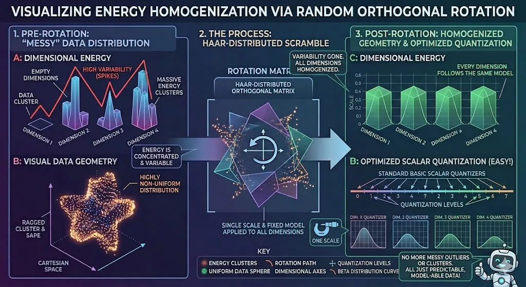
So the quantizer doesn’t need to guess. It doesn’t need to be complex. It just applies a simple, uniform rule. And it works perfectly.
Do you see the elegance here? We didn’t create a complex, advanced quantizer. No. We didn’t try to brute-force a difficult problem. Instead, we applied a simple, elegant mathematical transformation to change the nature of the data itself. We made the data easier to quantize. This is good engineering! We shifted the complexity from the quantizer to a pre-processing step, where we can solve the problem once with a simple, standard rotation matrix.
We didn’t change what the model weights are, just how we choose to look at them. And that difference is everything. It makes the impossible possible. It’s beautiful. That’s what’s happening.
Stage One: PolarQuant and Geometric Mapping
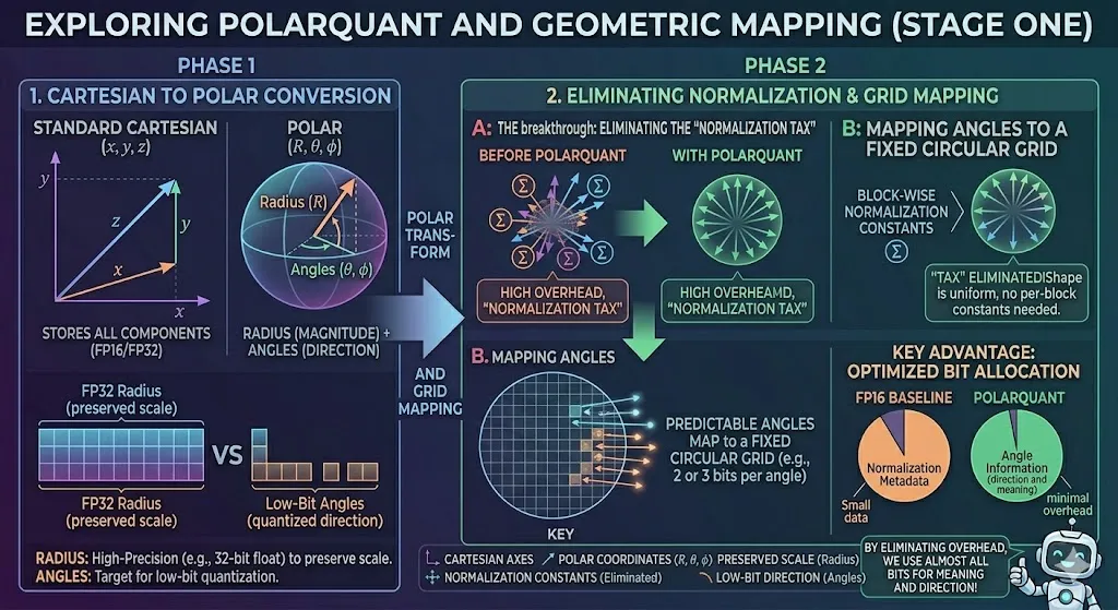
The first stage of the pipeline utilizes PolarQuant Rather than using standard Cartesian coordinates to map high-dimensional space, PolarQuant converts vectors into polar coordinates consisting of a radius and a set of angles. In this geometric representation:
The Radius represents the data’s “strength” or magnitude. TurboQuant typically stores these radii with high precision (e.g., as 32-bit floats) to preserve the scale.
The Angles represent the direction and meaning of the vector. Because the earlier random rotation has already made the distribution of these angles highly concentrated and predictable, the system can map them onto a fixed, circular grid. The breakthrough here is the elimination of the “normalization tax.” Because the “shape” of the data is now known and uniform, the model no longer needs to store expensive, block-wise normalization constants. This allows PolarQuant to use the majority of its bit budget (e.g., 2 or 3 bits) to capture the main concept and direction of the original vector with minimal overhead. **
Let’s look at this diagram and decode what is actually happening when it says “Standard Cartesian to Polar conversion” in this PolarQuant paper. We saw earlier that we applied that random rotation—that “mathematical scramble”—to make the messy data uniform and concentrated. That was a pre-processing step.
The Fundamental Shift: Cartesian vs. Polar
On the left, we have the “STANDARD CARTESIAN (x, y, z)” coordinate system. This is what we are all used to. Every vector—every point in that high-dimensional space—is just a bunch of numbers: an x-value, a y-value, a z-value. If you are a computer trying to compress this, what do you see? You see a massive set of components (the components part is key) that are stored with full precision. The diagram calls it “(FP16/FP32)”. This is how you make a heavy model. You are carrying a lot of redundant information in every axis.
Now, look at what PolarQuant does! It says, “Forget the individual axes, we are going geometric.” It converts that exact same vector from Cartesian into Polar coordinates (R,theta,phi). This is a transformation. You are changing your perspective.
And what does this geometric perspective give you? Look at that sphere. We split the single concept of “the vector” into two separate and distinct properties.
1. The Radius: Storing Magnitude
Look at that “Radius (R)” arrow, pointing straight up. What is that? In geometry, the radius represents the data’s “strength” or “magnitude”. It is the fundamental scale of the information. This is critical data. And because it is so critical, look at how we store it. We don’t quantize it heavily. No. TurboQuant stores these radii with high precision—32-bit floats—to preserve the scale.
Look at the storage comparison box at the bottom: “FP32 Radius (preserved scale)” is a large, solid block. We aren’t being cheap with memory here. Why? Because you cannot lose the magnitude information. If you do, you lose the fundamental concept of the data. Good engineers understand which components are not negotiable.
2. The Angles: Mapping to a Grid
But what about the angles? Those are (theta,phi). They represent the vector’s direction and meaning. This is the “concept” of the data, the direction it points in semantic space.
And this is where that earlier random rotation pays off! Remember that scramble? It made the distribution of these angles highly concentrated and predictable. If the distribution is predictable, that is engineering gold. Because then you can map them perfectly onto a fixed, circular grid.
Look at Panel B on the right: “MAPPING ANGLES TO A FIXED CIRCULAR GRID”. We have this beautiful, uniform grid with specific bins (small squares) and we are just mapping those glowing data points (the predictable angle arrows) directly into the grid.
And what does this mean for memory? Look at that storage box: “Low-Bit Angles (quantized direction)”. They are small blocks! Why? Because we have made the angles so easy to model that we can quantize them to as little as 2 or 3 bits per angle and still capture the main concept and direction of the original vector.
The Real Engineering Breakthrough: Eliminating the “Normalization Tax”
Let’s break it down.
On the left, we have the “BEFORE POLARQUANT” state. Look at what you have to do to make this spiky, Cartesian data usable in an LLM. You have multiple distinct clusters of vectors (the vector groups with the Sigma sum symbols). To use these, you must normalize them.
And how do you do it? Look at the diagram’s label: “TAX” . This is what engineers call a penalty. For every single one of those blocks—for every cluster of data—you must store expensive, block-wise normalization constants. Every block needs its own specific constant. This is high overhead! You are paying a heavy memory penalty, carrying all this extra baggage (the “metadata”), just to normalize every little piece of your data before you can use it. That is inefficient. That is a bad design.
The PolarQuant Solution: Uniform Geometry
Now, look at the other side, “WITH POLARQUANT”. Remember that geometric perspective change we did? Our geometric scramble has already solved the problem for us. By changing our perspective, we have already made the “shape” of the angle data uniform and concentrated.
Look at that perfect, uniform sphere of vectors! We forced the geometry itself into this known, symmetric shape.
Because we did that, we eliminate the entire “Normalization Tax.” The diagram literally says: ‘“TAX” ELIMINATED!Shape is uniform, no per-block constants needed.’ Why do we not need them? Because every single piece of data now shares the same known normalization property! The data is normalized by the very geometry we created. You carry no baggage. The overhead is gone. Good engineering eliminates redundant tasks.
The Purity of Bit Budget
And what does this mean for us as engineers? It frees up your bit budget! Look at that final pie chart comparison, which is absolute poetry.
Look at that optimization. We eliminated the metadata overhead. Now we can dedicate almost all of our precious bit budget—even if it’s just 2-3 bits—to capturing the main concept and meaning of the original vector.
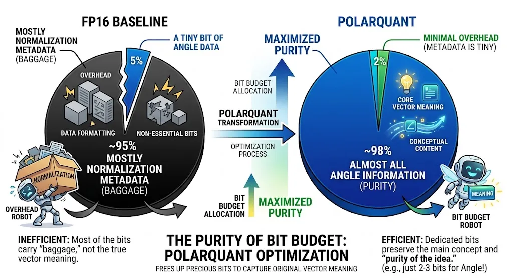
Do you see the elegance? We didn’t change what the vector is. No. We just changed how we store it. And that change allows us to carry almost no baggage, dedicating all of our precious resources to preserving the meaning, the purity of the idea. The little robot on the diagram is smiling for a reason. That’s good engineering!
Stage Two: Correcting the Residual with QJL
Even with the efficiency of PolarQuant, a tiny amount of “rounding error” or residual remains. In the context of the attention mechanism, these small errors can lead to “biased” inner product estimates, which are the core of how LLMs determine relevance between words.
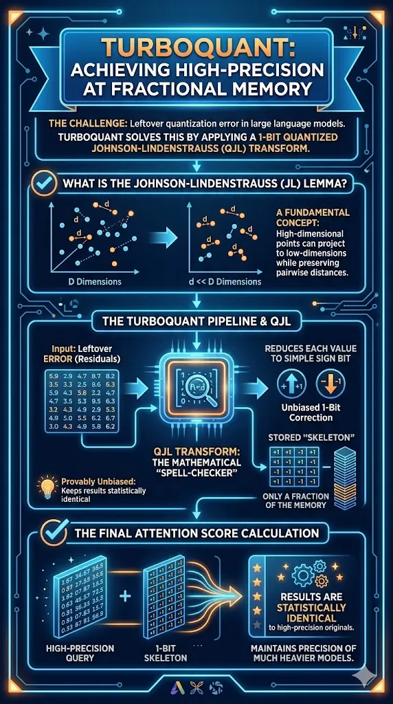
Everyone wants to squeeze them onto smaller and cheaper hardware. But when you compress—or quantize—the model weights and the context, you introduce noise. Errors. Leftover ‘residuals’ that ruin your accuracy. And this is exactly what TurboQuant tackles, using some real, heavy-duty math!
Here’s the problem: when we store the KV cache—which is like the model’s short-term memory—it takes up massive amounts of VRAM. People are trying 8-bit quantization, even 4-bit, and even then, sometimes the model just falls apart. There’s just too much error.
Section 2: Show Me The Proof (The Theory)
The researchers didn’t just guess this works. They went all-in on information theory and proved that TurboQuant is incredibly efficient—it’s within about 2.7x of the Shannon limit, the absolute physical minimum amount of information required for a given distortion.
And look at this table on MSE Distortion. This is what solidifies everything.
1-bit quantization (per channel)? Your distortion (MSE) is high (approx 0.36), and the model is basically broken. Significant logic degradation. You can’t just quantize KV cache to 1-bit and expect it to work.
2-bit? Okay, better. Distortion drops a lot (approx 0.117). The accuracy impact is now just marginal degradation. This is getting interesting.
3-bit? Look at this jump approx 0.03 MSE. We are talking near-zero loss.
4-bit? 0.009 MSE. Absolute Quality Neutrality. The model is indistinguishable from the high-precision base model, but using 4-bit per channel instead of 16-bit.
These findings show that we don’t need high-precision data to get high-precision attention scores! We can achieve zero quality loss for things like KV cache quantization with only around 3.5 bits per channel.
This is exactly how TurboQuant works. It’s combining a clever low-bit representation (the high-precision query and a simple stored skeleton) with a massive theoretical foundation to break the memory bottleneck. That’s why this is so huge for the future of deploying these massive models.
Performance Benchmarks: The “Needle-in-a-Haystack” Test
The ultimate test of any compression algorithm for LLMs is its performance on long-context benchmarks. One such test is “Needle-in-a-Haystack,” which hides a specific sentence inside 100,000 words to see if the model can find it. In testing across models like Llama-3.1-8B and Mistral-7B, TurboQuant achieved perfect recall scores, mirroring the performance of uncompressed models while reducing the KV cache memory footprint by at least 6x. Beyond chatbot memory, TurboQuant is transformative for semantic search. Modern search engines increasingly rely on comparing the meanings of billions of vectors rather than matching keywords. TurboQuant achieves superior recall ratios compared to state-of-the-art methods like Product Quantization (PQ), all while reducing indexing time to virtually zero because it does not require an offline training phase.
Hardware Acceleration on NVIDIA H100
On high-end hardware like the NVIDIA H100 GPU, the implementation of 4-bit TurboQuant provides an 8x performance boost in computing attention logs. This speedup occurs because the reduced memory footprint allows for much faster data transfer between the HBM and SRAM.
The Catch: Computational Costs and Implementation Challenges
In software engineering, there is no such thing as a “free lunch,” and TurboQuant is no exception. While it provides massive memory savings, it introduces its own set of challenges—what an engineer might call “the catch”.
The Cost of Scrambling
The first challenge is the computational cost of the random rotation. While the rotation simplifies the geometry for compression, the rotation itself is a matrix-vector multiplication (O(d^2)), which adds a runtime step to the quantization process. In some scenarios, this extra step might be expensive for on-the-fly cache quantization.
Fidelity vs. Speed on Unified Memory
Early adopters using next-generation hardware like the NVIDIA Grace Blackwell (GB10) have noted that while TurboQuant helps bypass RAM bandwidth limitations, it can lead to stability issues and information loss if not implemented carefully. For production-grade reliability, the cosine similarity of compressed vectors must remain above a 0.98 threshold. Some initial tests showed similarity dropping to ~0.89, suggesting that “hand-written” CUDA kernels may no longer be sufficient. The community is increasingly moving toward Triton, which JIT-compiles kernels tailored to the specific microarchitecture, as the only way to bypass driver-level compatibility pitfalls and achieve the full theoretical speedup.
Market Impact: The Semiconductor Plunge
The announcement of TurboQuant on March 24, 2026, sent shockwaves through the global semiconductor industry, illustrating just how sensitive the market is to AI efficiency breakthroughs. Within hours, stock prices for major memory chip manufacturers like Samsung, SK Hynix, and Micron plummeted.
Demand Concerns: Investors feared that if TurboQuant could reduce memory demand by 6x, the industry’s record-high DRAM and HBM prices would collapse as fewer chips would be needed to achieve the same AI performance.
Profit-Taking: Analysts also attributed the selloff to profit-taking in a cyclical sector that had gained nearly 200% the previous year.
The Counter-Argument (Jevons’ Paradox): Other researchers suggested that resolving memory bottlenecks would actually increase demand for chips. By making it cheaper to run models, more companies would adopt AI for more complex tasks (like spatiotemporal transformers for high-res video), potentially driving a paradoxical increase in total memory consumption.
Architectural Implications for the Future of AI
TurboQuant, along with PolarQuant and QJL, represents more than just a performance trick; these are fundamental algorithmic contributions backed by strong theoretical proofs. They operate near the theoretical lower bounds of what is mathematically possible in data compression.
Semantic Search at Scale
As web search shifts from keyword matching to semantic understanding, the ability to query large vector indices with minimal memory and near-zero preprocessing becomes critical. TurboQuant allows search engines to handle massive vector sets with the efficiency of a 3-bit system while maintaining state-of-the-art accuracy.
3 bit or 4 bit
TurboQuant is designed to function primarily as a 3-bit quantization method for Key-Value (KV) caches in large language models, offering 6x memory reduction without sacrificing accuracy. However, it can operate in 4-bit mode to achieve up to 8x faster attention computation on NVIDIA H100 GPUs. Build Fast with AI
3-bit Precision (Core Capability): TurboQuant compresses the KV cache down to 3 bits per value, allowing for at least 6x reduction in memory footprint without needing retraining or fine-tuning.
4-bit Performance: When operating at 4-bit, the method delivers optimal speedup, with tests showing an 8x increase in computing attention logs compared to 32-bit unquantized keys.
On-Device and Edge AI
For the global consumer electronics industry, TurboQuant offers a path to powerful “on-device” AI. By shrinking the memory bottleneck, smartphones and laptops can retain more context for longer conversations without relying on expensive, high-bandwidth memory. This could stabilize consumer electronics prices by reducing the reliance on a limited global supply of HBM.
Conclusions: The New Efficiency Standard
The genius of Google’s TurboQuant lies in its recognition that the “memory wall” is a problem of geometry and bias as much as it is a problem of hardware capacity. By starting from first principles—scrambling the data to achieve a uniform distribution, utilizing polar coordinates to eliminate metadata overhead, and applying 1-bit QJL to fix residual bias—TurboQuant has redefined what is possible in AI efficiency.
For software engineers and backend architects, the lesson is clear: to build the next generation of scalable AI, one must “swim with the tide” of the technology, understanding its internal bottlenecks and building around its strengths rather than fighting its limitations. As TurboQuant moves from research to production, it will likely become the foundational technique for everything from real-time interactive pipelines in ComfyUI to massive semantic search engines, proving that sometimes, the most effective way to go “bigger” is to go much, much smaller.