Video coming soon. Start with the reading below.
At the internet layer, the communication between two nodes happens by routing packets to their destination from one router to the next. Two ingredients are required for this: a way to address nodes and a mechanism to route packets across routers.
Addressing is handled by the IP protocol. For example, IPv6 provides a 128-bit address space, allowing 2128 addresses. To decide where to send a packet, a router needs to consult a local routing table. The table maps a destination address to the address of the next router along the path to that destination. The responsibility of building and communicating the routing tables across routers lies with the Border Gateway Protocol (BGP[1]).
Now, IP doesn’t guarantee that data sent over the internet will arrive at its destination. For example, if a router becomes overloaded, it might start dropping packets. This is where TCP[2] comes in, a transport-layer protocol that exposes a reliable communication channel between two processes on top of IP. TCP guarantees that a stream of bytes arrives in order without gaps, duplication, or corruption. TCP also implements a set of stability patterns to avoid overwhelming the network and the receiver.
Reliability
To create the illusion of a reliable channel, TCP partitions a byte stream into discrete packets called segments. The segments are sequentially numbered, which allows the receiver to detect holes and duplicates. Every segment sent needs to be acknowledged by the receiver. When that doesn’t happen, a timer fires on the sending side and the segment is retransmitted. To ensure that the data hasn’t been corrupted in transit, the receiver uses a checksum to verify the integrity of a delivered segment.
Connection lifecycle
A connection needs to be opened before any data can be transmitted on a TCP channel. The operating system manages the connection state on both ends through a socket. The socket keeps track of the state changes of the connection during its lifetime. At a high level, there are three states the connection can be in:
- The opening state in which the connection is being created.
- The established state in which the connection is open and data is being transferred.
- The closing state in which the connection is being closed.
In reality, this is a simplification, as there are more states[3] than the three above.
A server must be listening for connection requests from clients before a connection is established. TCP uses a three-way handshake to create a new connection, as shown in Figure 2.1:
- The sender picks a random sequence number x and sends a SYN segment to the receiver.
- The receiver increments x, chooses a random sequence number y, and sends back a SYN/ACK segment.
- The sender increments both sequence numbers and replies with an ACK segment and the first bytes of application data.
The sequence numbers are used by TCP to ensure the data is delivered in order and without holes.
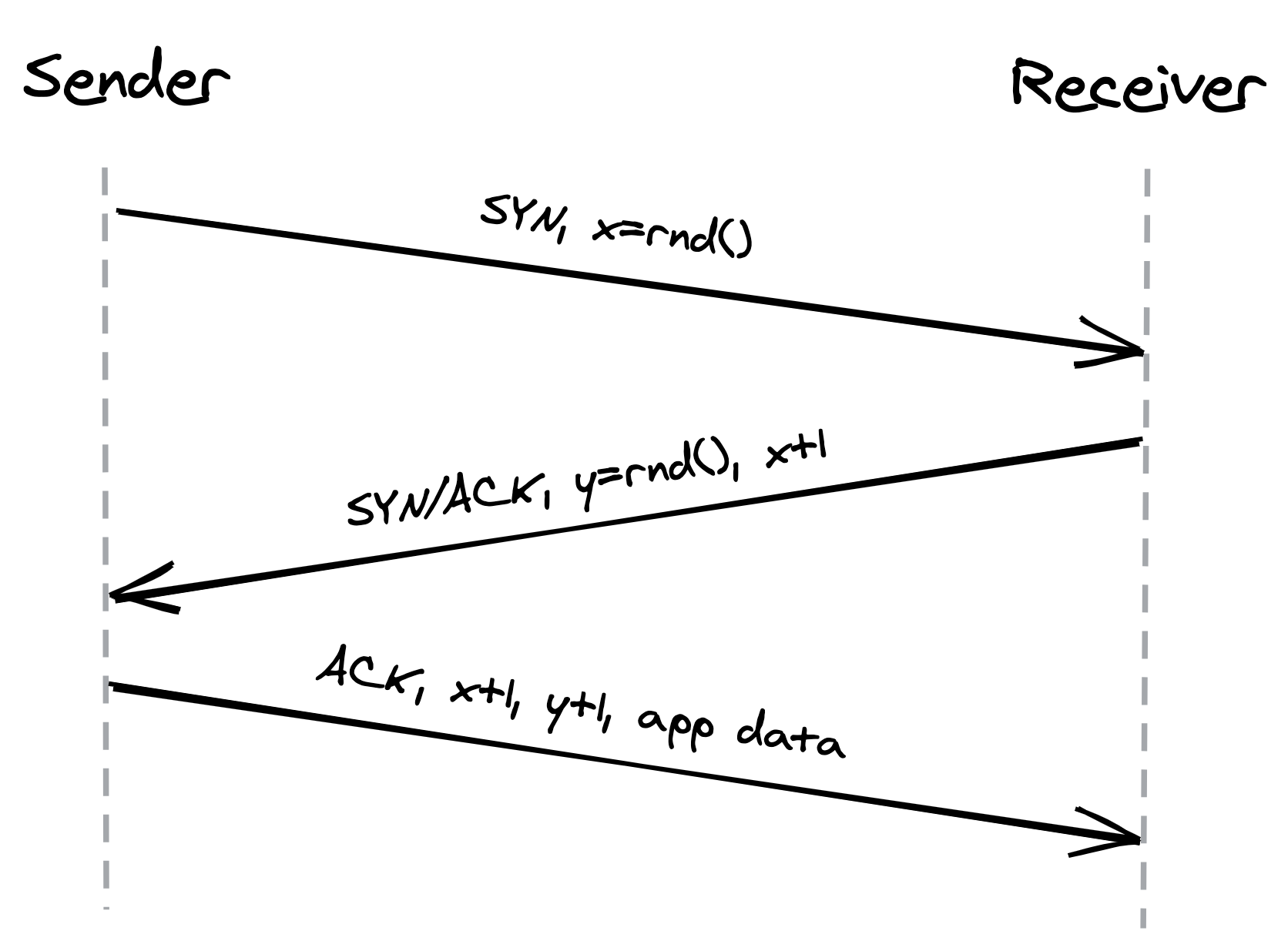
Figure 2.1: Three-way handshake
The handshake introduces a full round-trip in which no application data is sent. So until the connection has been opened, the bandwidth is essentially zero. The lower the round trip time is, the faster the connection can be established. Therefore, putting servers closer to the clients helps reduce this cold-start penalty.
After the data transmission is complete, the connection needs to be closed to release all resources on both ends. This termination phase involves multiple round-trips. If it’s likely that another transmission will occur soon, it makes sense to keep the connection open to avoid paying the cold-start tax again.
Moreover, closing a socket doesn’t dispose of it immediately as it transitions to a waiting state (TIME_WAIT) that lasts several minutes and discards any segments received during the wait. The wait prevents delayed segments from a closed connection from being considered part of a new connection. But if many connections open and close quickly, the number of sockets in the waiting state will continue to increase until it reaches the maximum number of sockets that can be open, causing new connection attempts to fail. This is another reason why processes typically maintain connection pools to avoid recreating connections repeatedly.
Flow control
Flow control is a backoff mechanism that TCP implements to prevent the sender from overwhelming the receiver. The receiver stores incoming TCP segments waiting to be processed by the application into a receive buffer, as shown in Figure 2.2.
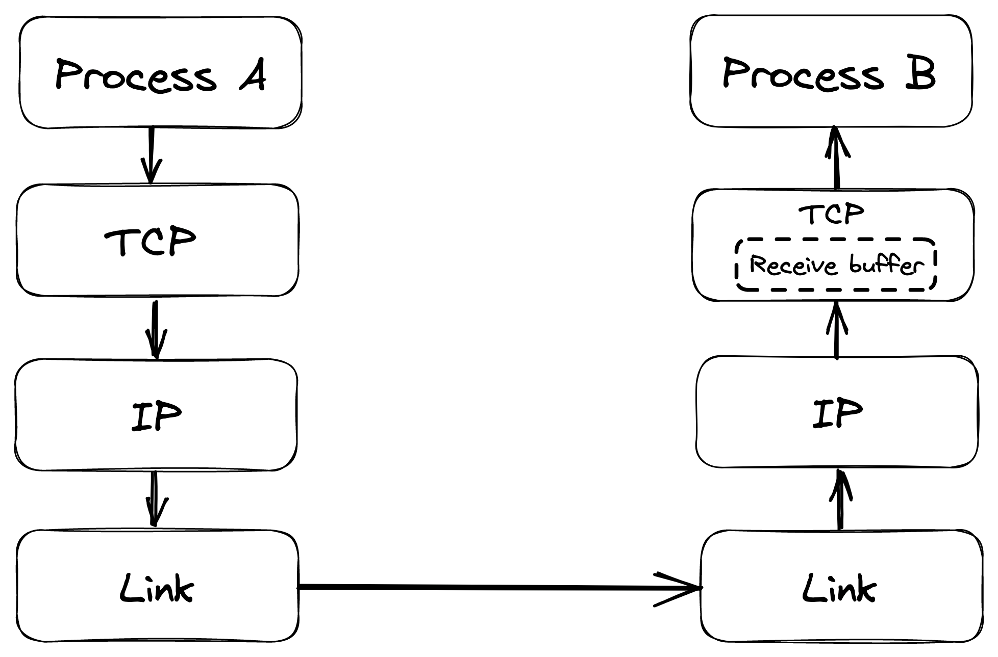
Figure 2.2: The receive buffer stores data that hasn’t yet been processed by the destination process.
The receiver also communicates the size of the buffer to the sender whenever it acknowledges a segment, as shown in Figure 2.3.
Assuming it’s respecting the protocol, the sender avoids sending more data than can fit in the receiver’s buffer.
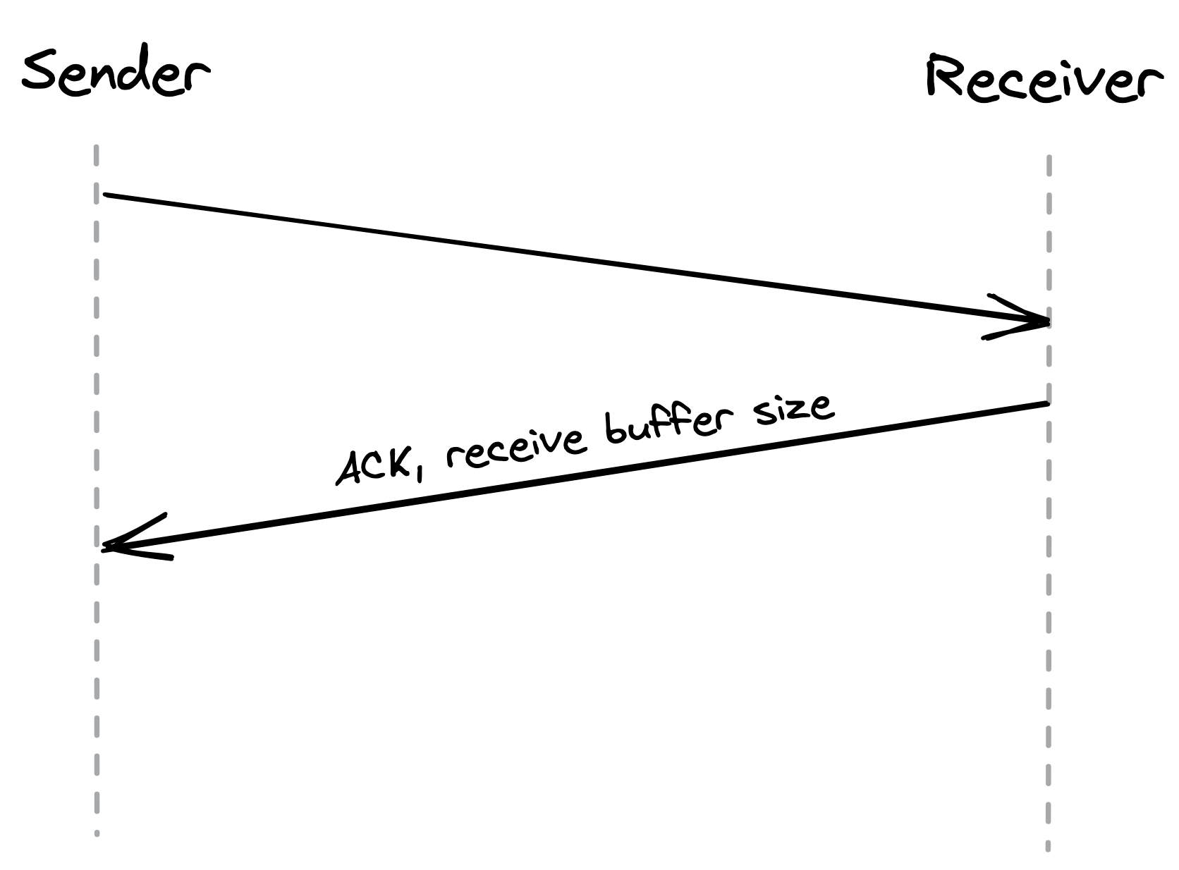
Figure 2.3: The size of the receive buffer is communicated in the headers of acknowledgment segments.
This mechanism is not too dissimilar to rate-limiting at the service level, a mechanism that rejects a request when a specific quota is exceeded (see Rate-limiting in Upstream resiliency). But, rather than rate-limiting on an API key or IP address, TCP is rate-limiting on a connection level.
Congestion control
TCP guards not only against overwhelming the receiver, but also against flooding the underlying network. The sender maintains a so-called congestion window, which represents the total number of outstanding segments that can be sent without an acknowledgment from the other side. The smaller the congestion window is, the fewer bytes can be in flight at any given time, and the less bandwidth is utilized.
When a new connection is established, the size of the congestion window is set to a system default. Then, for every segment acknowledged, the window increases its size exponentially until it reaches an upper limit. This means we can’t use the network’s full capacity right after a connection is established. The shorter the round-trip time (RTT), the quicker the sender can start utilizing the underlying network’s bandwidth, as shown in Figure 2.4.
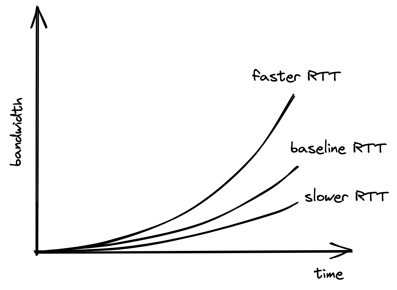
Figure 2.4: The shorter the RTT, the quicker the sender can start utilizing the underlying network’s bandwidth.
What happens if a segment is lost? When the sender detects a missed acknowledgment through a timeout, a mechanism called congestion avoidance kicks in, and the congestion window size is reduced. From there onwards, the passing of time increases the window size[4] by a certain amount, and timeouts decrease it by another.
As mentioned earlier, the size of the congestion window defines the maximum number of bytes that can be sent without receiving an acknowledgment. Because the sender needs to wait for a full round trip to get an acknowledgment, we can derive the maximum theoretical bandwidth by dividing the size of the congestion window by the round trip time:
Bandwidth = WinSize / RTT
The equation[5] shows that bandwidth is a function of latency. TCP will try very hard to optimize the window size since it can’t do anything about the round-trip time. However, that doesn’t always yield the optimal configuration. Due to the way congestion control works, the shorter the round-trip time, the better the underlying network’s bandwidth is utilized. This is more reason to put servers geographically close to the clients.
Custom protocols
TCP’s reliability and stability come at the price of lower bandwidth and higher latencies than the underlying network can deliver. If we drop the stability and reliability mechanisms that TCP provides, what we get is a simple protocol named User Datagram Protocol[6] (UDP) — a connectionless transport layer protocol that can be used as an alternative to TCP.
Unlike TCP, UDP does not expose the abstraction of a byte stream to its clients. As a result, clients can only send discrete packets with a limited size called datagrams. UDP doesn’t offer any reliability as datagrams don’t have sequence numbers and are not acknowledged. UDP doesn’t implement flow and congestion control either. Overall, UDP is a lean and bare-bones protocol. It’s used to bootstrap custom protocols, which provide some, but not all, of the stability and reliability guarantees that TCP does[7].
For example, in multiplayer games, clients sample gamepad events several times per second and send them to a server that keeps track of the global game state. Similarly, the server samples the game state several times per second and sends these snapshots back to the clients. If a snapshot is lost in transmission, there is no value in retransmitting it as the game evolves in real-time; by the time the retransmitted snapshot would get to the destination, it would be obsolete. This is a use case where UDP shines; in contrast, TCP would attempt to redeliver the missing data and degrade the game’s experience.
References
- “RFC 4271: A Border Gateway Protocol 4 (BGP-4),” https://datatracker.ietf.org/doc/html/rfc4271
- “RFC 793: Transmission Control Protocol,” https://tools.ietf.org/html/rfc793
- “TCP State Diagram,” https://en.wikipedia.org/wiki/Transmission_Control_Protocol#/media/File:Tcp_state_diagram_fixed_new.svg
- “CUBIC: A New TCP-Friendly High-Speed TCP Variant,” https://citeseerx.ist.psu.edu/viewdoc/download?doi=10.1.1.153.3152&rep=rep1&type=pdf
- “Bandwidth-delay product,” https://en.wikipedia.org/wiki/Bandwidth-delay_product
- “RFC 768: User Datagram Protocol,” https://datatracker.ietf.org/doc/html/rfc768
- As we will later see, HTTP 3 is based on UDP to avoid some of TCP’s short-comings.
