Video coming soon. Start with the reading below.
When an application’s data keeps growing in size, its volume will eventually become large enough that it can’t fit on a single machine. To work around that, it needs to be split into partitions, or shards, small enough to fit into individual nodes. As an additional benefit, the system’s capacity for handling requests increases as well, since the load of accessing the data is spread over more nodes.
When a client sends a request to a partitioned system, the request needs to be routed to the node(s) responsible for it. A gateway service (i.e., a reverse proxy) is usually in charge of this, knowing how the data is mapped to partitions and nodes (see Figure 16.1). This mapping is generally maintained by a fault-tolerant coordination service, like etcd or Zookeeper.
Partitioning is not a free lunch since it introduces a fair amount of complexity:
- A gateway service is required to route requests to the right nodes.
- To roll up data across partitions, it needs to be pulled from multiple partitions and aggregated (e.g., think of the complexity of implementing a “group by” operation across partitions).
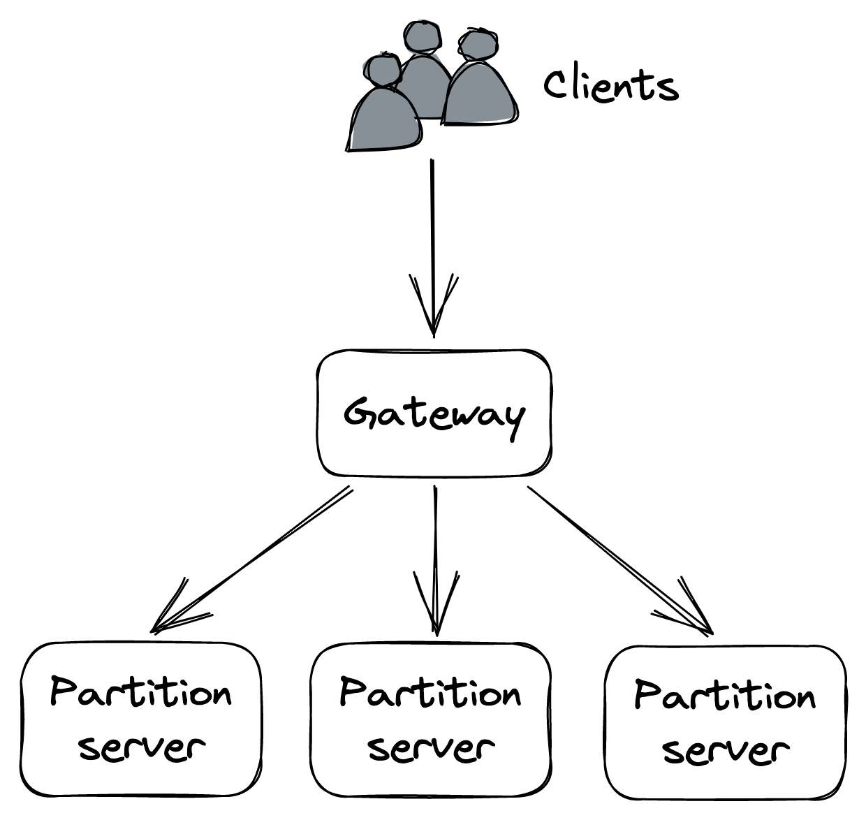
Figure 16.1: A partitioned application with a gateway that routes requests to partitions
- Transactions are required to atomically update data that spans multiple partitions, limiting scalability.
- If a partition is accessed much more frequently than others, the system’s ability to scale is limited.
- Adding or removing partitions at run time becomes challenging, since it requires moving data across nodes.
It’s no coincidence we are talking about partitioning right after discussing CDNs. A cache lends itself well to partitioning as it avoids most of this complexity. For example, it generally doesn’t need to atomically update data across partitions or perform aggregations spanning multiple partitions.
Now that we have an idea of what partitioning is and why it’s useful, let’s discuss how data, in the form of key-value pairs, can be mapped to partitions. At a high level, there are two main ways of doing that, referred to as range partitioning and hash partitioning. An important prerequisite for both is that the number of possible keys is very large; for example, a boolean key with only two possible values is not suited for partitioning since it allows for at most two partitions.
Range partitioning
Range partitioning splits the data by key range into lexicographically sorted partitions, as shown in Figure 16.2. To make range scans fast, each partition is generally stored in sorted order on disk.
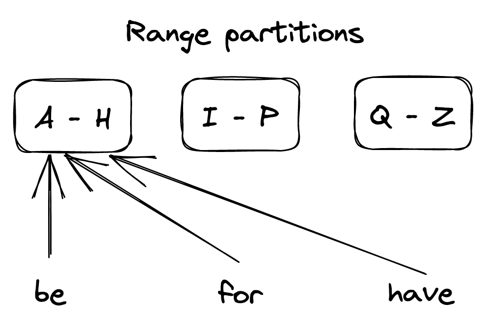
Figure 16.2: A range-partitioned dataset
The first challenge with range partitioning is picking the partition boundaries. For example, splitting the key range evenly makes sense if the distribution of keys is more or less uniform. If not, like in the English dictionary, the partitions will be unbalanced and some will have a lot more entries than others.
Another issue is that some access patterns can lead to hotspots, which affect performance. For example, if the data is range partitioned by date, all requests for the current day will be served by a single node. There are ways around that, like adding a random prefix to the partition keys, but there is a price to pay in terms of increased complexity.
When the size of the data or the number of requests becomes too large, the number of nodes needs to be increased to sustain the increase in load. Similarly, if the data shrinks and/or the number of requests drops, the number of nodes should be reduced to decrease costs. The process of adding and removing nodes to balance the system’s load is called rebalancing. Rebalancing has to be implemented in a way that minimizes disruption to the system, which needs to continue to serve requests. Hence, the amount of data transferred when rebalancing partitions should be minimized.
One solution is to create a lot more partitions than necessary when the system is first initialized and assign multiple partitions to each node. This approach is also called static partitioning since the number of partitions doesn’t change over time. When a new node joins, some partitions move from the existing nodes to the new one so that the store is always in a balanced state. The drawback of this approach is that the number of partitions is fixed and can’t be easily changed. Getting the number of partitions right is hard — too many partitions add overhead and decrease performance, while too few partitions limit scalability. Also, some partitions might end up being accessed much more than others, creating hotspots.
The alternative is to create partitions on demand, also referred to as dynamic partitioning. The system starts with a single partition, and when it grows above a certain size or becomes too hot, the partition is split into two sub-partitions, each containing approximately half of the data, and one of the sub-partitions is transferred to a new node. Similarly, when two adjacent partitions become small or “cold” enough, they can be merged into a single one.
Hash partitioning
Let’s take a look at an alternative way of mapping data to partitions. The idea is to use a hash function that deterministically maps a key (string) to a seemingly random number (a hash) within a certain range (e.g., 0 and 264 −1). This guarantees that the keys’ hashes are distributed uniformly across the range.
Next, we assign a subset of the hashes to each partition, as shown in Figure 16.3. For example, one way of doing that is by taking the modulo of a hash, i.e., hash(key) mod N, where N is the number of partitions.
Although this approach ensures that the partitions contain more
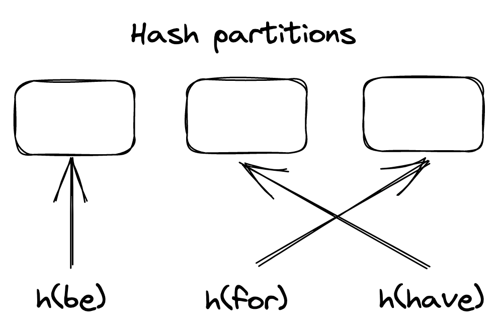
Figure 16.3: A hash-partitioned dataset
or less the same number of entries, it doesn’t eliminate hotspots if the access pattern is not uniform. For example, if a single key is accessed significantly more often than others, the node hosting the partition it belongs to could become overloaded. In this case, the partition needs to be split further by increasing the total number of partitions. Alternatively, the key needs to be split into sub-keys by, e.g., prepending a random prefix.
Assigning hashes to partitions via the modulo operator can become problematic when a new partition is added, as most keys have to be moved (or shuffled) to a different partition because their assignment changed. Shuffling data is extremely expensive as it consumes network bandwidth and other resources. Ideally, if a partition is added, only K
Nkeys should be shuffled around, where Kis the number of keys and Nis the number of partitions. One widely used hashing strategy with that property is consistent hashing.
With consistent hashing[1], a hash function randomly maps both the partition identifiers and keys onto a circle, and each key is assigned to the closest partition that appears on the circle in clockwise order (see Figure 16.4).
Now, when a new partition is added, only the keys that now map
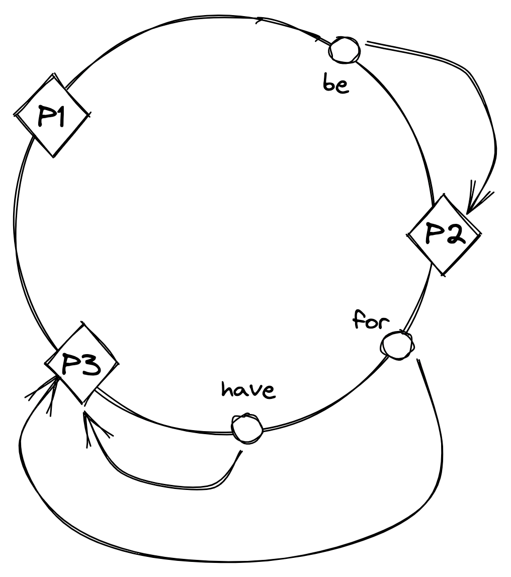
Figure 16.4: With consistent hashing, partition identifiers and keys are randomly distributed around a circle, and each key is assigned to the next partition that appears on the circle in clockwise order.
to it on the circle need to be reassigned, as shown in Figure 16.5.
The main drawback of hash partitioning compared to range partitioning is that the sort order over the partitions is lost, which is required to efficiently scan all the data in order. However, the data within an individual partition can still be sorted based on a secondary key.
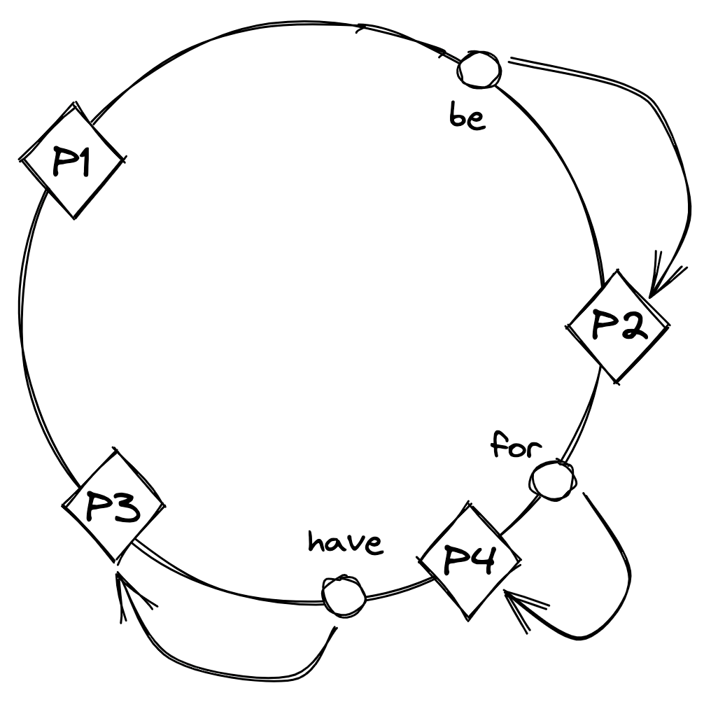
Figure 16.5: After partition P4 is added, the key ’for’ is reassigned to P4, but the assignment of the other keys doesn’t change.
References
- “Consistent Hashing and Random Trees: Distributed Caching Protocols for Relieving Hot Spots on the World Wide Web,” https://www.cs.princeton.edu/courses/archive/fall09/cos518/papers/chash.pdf