Study one concept at a time. Open the guided module →
Scalability
Overview: Scalability
Video coming soon. Start with the reading below.
“Treat servers like cattle, not pets.”
– Bill Baker
Over the last few decades, the number of people with access to the internet has steadily climbed. In 1996, only 1% of people worldwide had access to the internet, while today, it’s over 65%. In turn, this has increased the total addressable market of online businesses and led to the need for scalable systems that can handle millions of concurrent users.
For an application to scale, it must run without performance degradations as load increases. And as mentioned in Introduction (lesson 01.01), the only long-term solution for increasing the application’s capacity is to architect it so that it can scale horizontally.
In this part, we will walk through the journey of scaling a simple CRUD web application called Cruder. Cruder is comprised of a single-page JavaScript application that communicates with an application server through a RESTful HTTP API. The server uses the local disk to store large files, like images and videos, and a relational database to persist the application’s state. Both the database and the application server are hosted on the same machine, which is managed by a compute platform like AWS EC2. Also, the server’s public IP address is advertised by a managed DNS service, like AWS Route 53[14].
Users interact with Cruder through their browsers. Typically, a browser issues a DNS request to resolve the domain name to an IP address (if it doesn’t have it cached already), opens a TLS connection with the server, and sends its first HTTP GET request to it (see Figure 13.2).
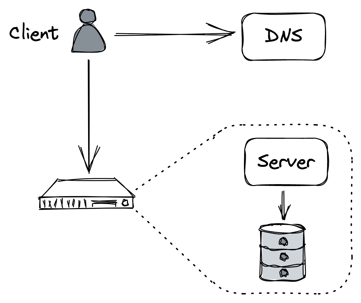
Figure 13.2: Cruder’s architecture
Although this architecture is good enough for a proof of concept, it’s not scalable or fault-tolerant. Of course, not all applications need to be highly available and scalable, but since you are reading this module to learn how such applications are built, we can assume that the application’s backend will eventually need to serve millions of requests per second.
And so, as the number of requests grows, the application server will require more resources (e.g., CPU, memory, disk, network) and eventually reach its capacity, and its performance will start to degrade. Similarly, as the database stores more data and serves more queries, it will inevitably slow down as it competes for resources with the application server.
The simplest and quickest way to increase the capacity is to scale up the machine hosting the application. For example, we could:
- increase the number of threads capable of running simulta-
neously by provisioning more processors or cores, • increase disk throughput by provisioning more disks (RAID), • increase network throughput by provisioning more NICs, • reduce random disk access latency by provisioning solidstate disks (SSD), • or reduce page faults by provisioning more memory.
The caveat is that the application needs to be able to leverage the additional hardware at its disposal. For example, adding more cores to a single-threaded application will not make much difference. More importantly, when we’ve maxed out on the hardware front, the application will eventually hit a hard physical limit that we can’t overcome no matter how much money we are willing to throw at it.
The alternative to scaling up is to scale out by distributing the application across multiple nodes. Although this makes the application more complex, eventually it will pay off. For example, we can move the database to a dedicated machine as a first step. By doing that, we have increased the capacity of both the server and the database since they no longer have to compete for resources. This is an example of a more general pattern called functional decomposition: breaking down an application into separate components, each with its own well-defined responsibility (see Figure 13.3).
As we will repeatedly see in the following chapters, there are other two general patterns that we can exploit (and combine) to build scalable applications: splitting data into partitions and distributing them among nodes (partitioning) and replicating functionality or data across nodes, also known as horizontal scaling (replication). In the following chapters, we will explore techniques based on those patterns for further increasing Cruder’s capacity, which require increasingly more effort to exploit.
HTTP caching (lesson 04.02) discusses the use of client-side caching to reduce the number of requests hitting the application.
Content delivery networks (lesson 04.03) describes using a content delivery network (CDN), a geographically distributed network of managed reverse proxies,
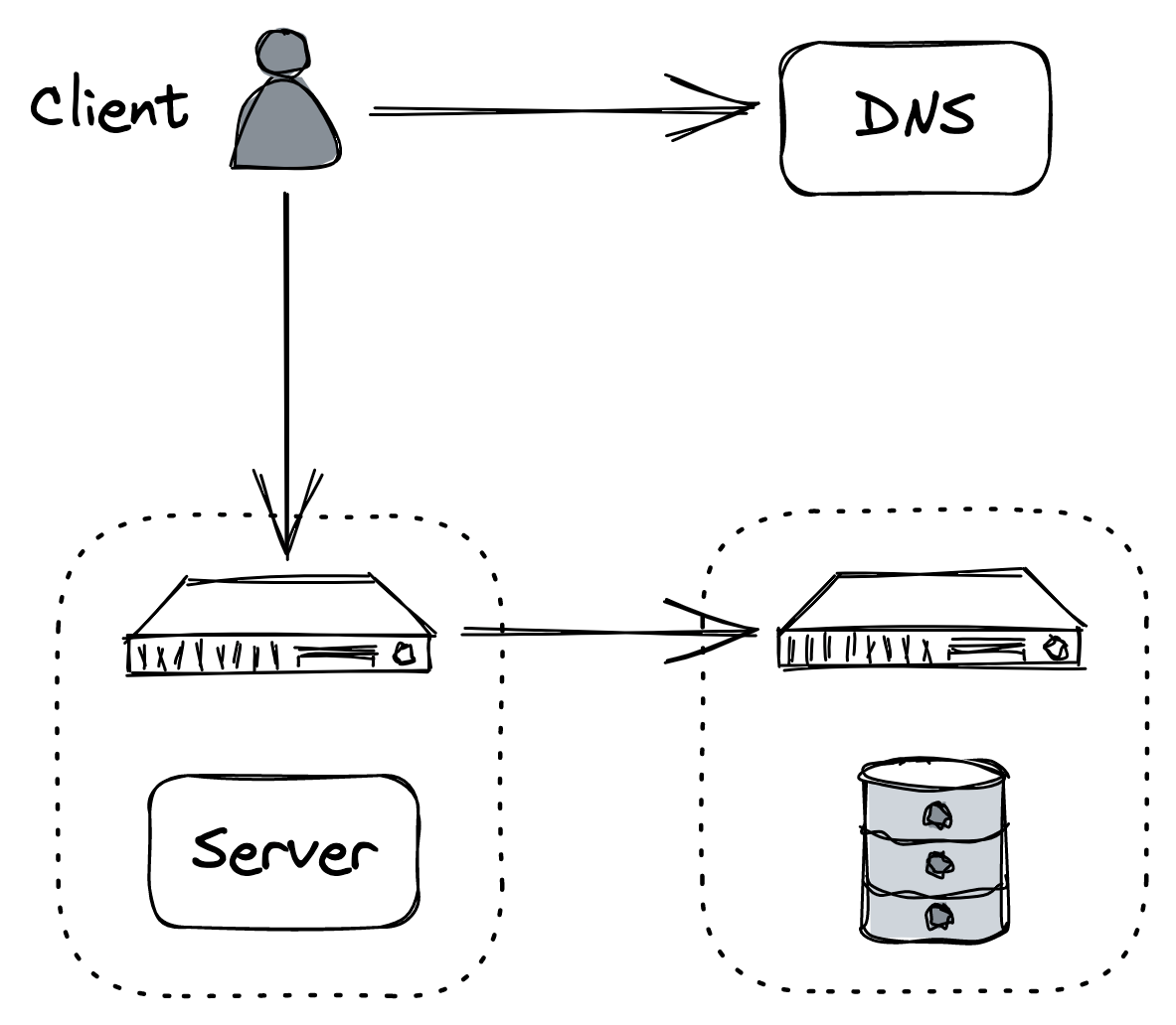
Figure 13.3: Moving the database to its own dedicated machine is an example of functional decomposition
to further reduce the number of requests the application needs to handle.
Partitioning (lesson 04.04) dives into partitioning, a technique used by CDNs, and pretty much any distributed data store, to handle large volumes of data. The chapter explores different partitioning strategies, such as range and hash partitioning, and the challenges that partitioning introduces.
File storage (lesson 04.05) discusses the benefits of offloading the storage of large static files, such as images and videos, to a managed file store. It then describes the architecture of Azure Storage, a highly available and scalable file store.
Network load balancing (lesson 04.06) talks about how to increase the application’s capacity by load-balancing requests across a pool of servers. The chapter starts with a simple approach based on DNS and then explores more flexible solutions that operate at the transport and application layers of the network stack.
Data storage (lesson 04.07) describes how to scale out the application’s relational database using replication and partitioning and the challenges that come with it. It then introduces NoSQL data stores as a solution to these challenges and recounts their evolution since their initial adoption in the industry.
Caching (lesson 04.08) takes a stab at discussing caching from a more general point of view by diving into the benefits and pitfalls of putting a cache in front of the application’s data store. Although caching is a deceptively simple technique, it can create subtle consistency and operational issues that are all too easy to dismiss.
Microservices (lesson 04.09) talks about scaling the development of the application across multiple teams by decomposing it into independently deployable services. Next, it introduces the concept of an API gateway as a means for external clients to communicate with the backend after it has been decomposed into separated services.
Control planes and data planes (lesson 04.10) describes the benefits of separating the serving of client requests (data plane) from the management of the system’s metadata and configuration (control plane), which is a common pattern in large-scale systems.
Messaging (lesson 04.11) explores the use of asynchronous messaging channels to decouple the communication between services, allowing two services to communicate even if one of them is temporarily unavailable. Messaging offers many other benefits, which we will explore in the chapter along with its best practices and pitfalls.
HTTP caching
Video coming soon. Start with the reading below.
Cruder’s application server handles both static and dynamic resources at this point. A static resource contains data that usually doesn’t change from one request to another, like a JavaScript or CSS file. Instead, a dynamic resource is generated by the server on the fly, like a JSON document containing the user’s profile.
Since a static resource doesn’t change often, it can be cached. The idea is to have a client (i.e., a browser) cache the resource for some time so that the next access doesn’t require a network call, reducing the load on the server and the response time.[1]
Let’s see how client-side HTTP caching works in practice with a concrete example. HTTP caching is limited to safe request methods that don’t alter the server’s state, like GET or HEAD. Suppose a client issues a GET request for a resource it hasn’t accessed before. The local cache intercepts the request, and if it can’t find the resource locally, it will go and fetch it from the origin server on behalf of the client.
The server uses specific HTTP response headers[2] to let clients know that a resource is cachable. So when the server responds with the resource, it adds a Cache-Control header that defines for how long to cache the resource (TTL) and an ETag header with a version identifier. Finally, when the cache receives the response, it stores the resource locally and returns it to the client (see Figure 14.1).
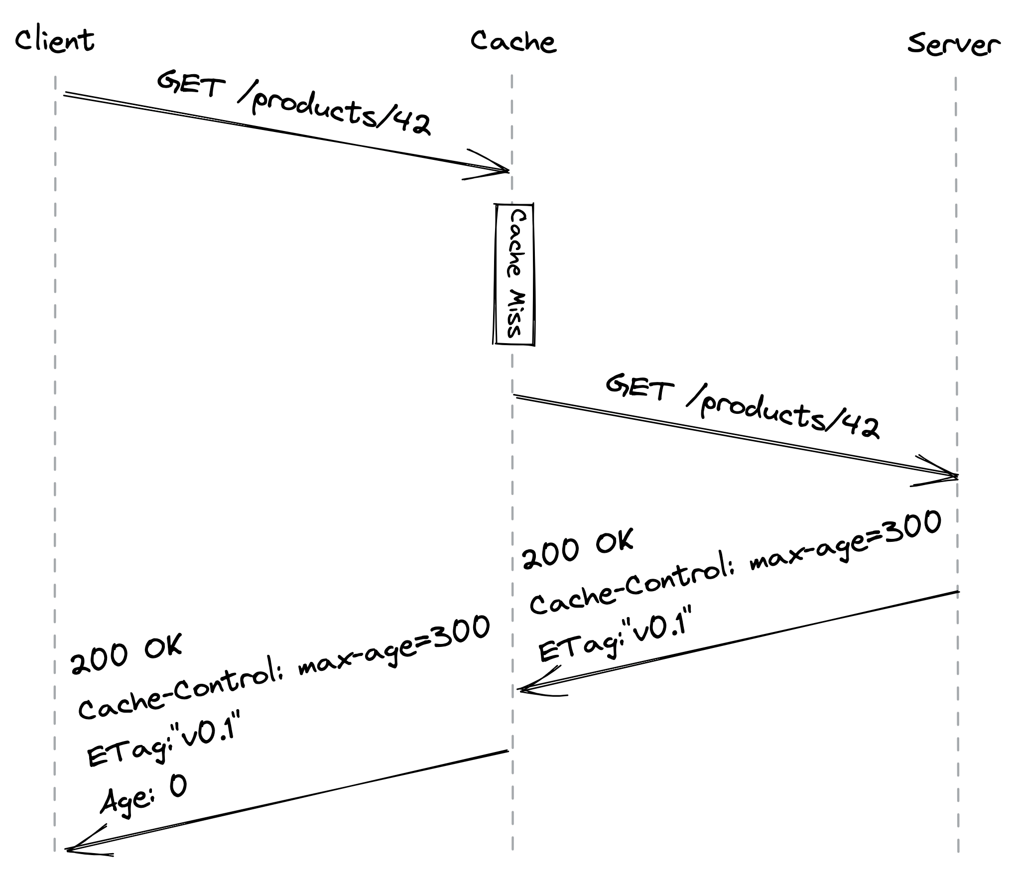
Figure 14.1: A client accessing a resource for the first time (the Age header contains the time in seconds the object was in the cache)
Now, suppose some time passes and the client tries to access the resource again. The cache first checks whether the resource hasn’t expired yet, i.e., whether it’s fresh. If so, the cache immediately returns it. However, even if the resource hasn’t expired from the client’s point of view, the server may have updated it in the meantime. That means reads are not strongly consistent, but we will safely assume that this is an acceptable tradeoff for our application.
If the resource has expired, it’s considered stale. In this case, the cache sends a GET request to the server with a conditional header (like If-None-Match) containing the version identifier of the stale resource to check whether a newer version is available. If there is, the server returns the updated resource; if not, the server replies with a 304 Not Modified status code (see Figure 14.2).
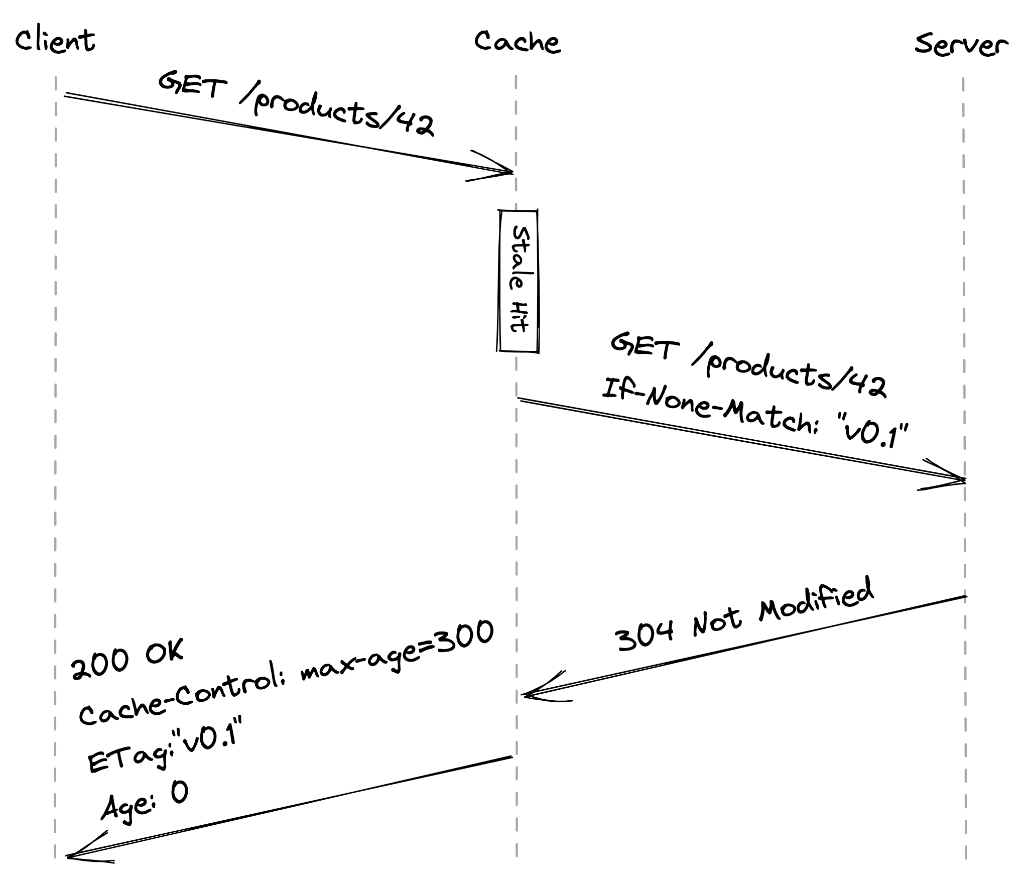
Figure 14.2: A client accessing a stale resource
Ideally, a static resource should be immutable so that clients can cache it “forever,” which corresponds to a maximum length of a year according to the HTTP specification. We can still modify a static resource if needed by creating a new one with a different URL so that clients will be forced to fetch it from the server.
Another advantage of treating static resources as immutable is that we can update multiple related resources atomically. For example, if we publish a new version of the application’s website, the updated HTML index file is going to reference the new URLs for the JavaScript and CSS bundles. Thus, a client will see either the old version of the website or the new one depending on which index file it has read, but never a mix of the two that uses, e.g., the old JavaScript bundle with the new CSS one.
Another way of thinking about HTTP caching is that we treat the read path (GET) differently from the write path (POST, PUT, DELETE) because we expect the number of reads to be several orders of magnitude higher than the number of writes. This is a common pattern referred to as the Command Query Responsibility Segregation[3] (CQRS) pattern.[4]
To summarize, allowing clients to cache static resources has reduced the load on our server, and all we had to do was to play with some HTTP headers! We can take caching one step further by introducing a server-side HTTP cache with a reverse proxy.
Reverse proxies
A reverse proxy is a server-side proxy that intercepts all communications with clients. Since the proxy is indistinguishable from the actual server, clients are unaware that they are communicating through an intermediary (see Figure 14.3).
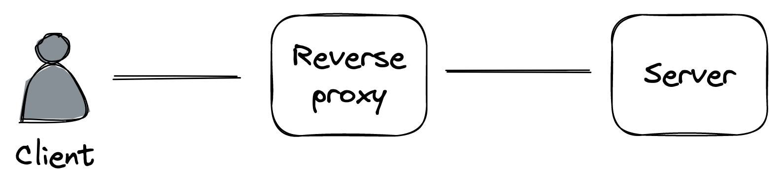
Figure 14.3: A reverse proxy acts as an intermediary between the clients and the servers.
A common use case for a reverse proxy is to cache static resources returned by the server. Since the cache is shared among the clients, it will decrease the load of the server a lot more than any client-side cache ever could.
Because a reverse proxy is a middleman, it can be used for much more than just caching. For example, it can:
- authenticate requests on behalf of the server;
- compress a response before returning it to the client to speed up the transmission;
- rate-limit requests coming from specific IPs or users to protect the server from being overwhelmed;
- load-balance requests across multiple servers to handle more load.
We will explore some of these use cases in the following lessons. NGINX[5] and HAProxy[6] are widely-used reverse proxies that we could leverage to build a server-side cache. However, many use cases for reverse proxies have been commoditized by managed services. So, rather than building out a server-side cache, we could just leverage a Content Delivery Network (CDN).
Content delivery networks
Video coming soon. Start with the reading below.
A CDN is an overlay network of geographically distributed caching servers (reverse proxies) architected around the design limitations of the network protocols that run the internet.
When using a CDN, clients hit URLs that resolve to caching servers that belong to the CDN. When a CDN server receives a request, it checks whether the requested resource is cached locally. If not, the CDN server transparently fetches it from the origin server (i.e., our application server) using the original URL, caches the response locally, and returns it to the client. AWS CloudFront[1] and Akamai[2] are examples of well-known CDN services.
Overlay network
You would think that the main benefit of a CDN is caching, but it’s actually the underlying network substrate. The public internet is composed of thousands of networks, and its core routing protocol, BGP, was not designed with performance in mind. It primarily uses the number of hops to cost how expensive a path is with respect to another, without considering their latencies or congestion.
As the name implies, a CDN is a network. More specifically, an overlay network[3] built on top of the internet that exploits a variety of techniques to reduce the response time of network requests and increase the bandwidth of data transfers.
When we first discussed TCP in Reliable links (lesson 02.02), we talked about the importance of minimizing the latency between a client and a server. No matter how fast the server is, if the client is located on the other side of the world from it, the response time is going to be over 100 ms just because of the network latency, which is physically limited by the speed of light. Not to mention the increased error rate when sending data across the public internet over long distances.
This is why CDN clusters are placed in multiple geographical locations to be closer to clients. But how do clients know which cluster is closest to them? One way is via global DNS load balancing[4]: an extension to DNS that considers the location of the client inferred from its IP, and returns a list of the geographically closest clusters taking into account also the network congestion and the clusters’ health.
CDN servers are also placed at internet exchange points, where ISPs connect to each other. That way, virtually the entire communication from the origin server to the clients flows over network links that are part of the CDN, and the brief hops on either end have low latencies due to their short distance.
The routing algorithms of the overlay network are optimized to select paths with reduced latencies and congestion, based on continuously updated data about the health of the network. Additionally, TCP optimizations are exploited where possible, such as using pools of persistent connections between servers to avoid the overhead of setting up new connections and using optimal TCP window sizes to maximize the effective bandwidth (see Figure 15.1).
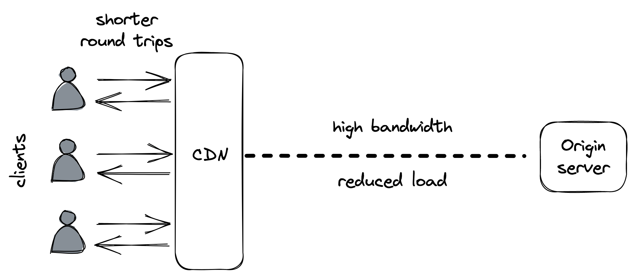
Figure 15.1: A CDN reduces the round trip time of network calls for clients and the load for the origin server.
The overlay network can also be used to speed up the delivery of dynamic resources that cannot be cached. In this capacity, the CDN becomes the frontend for the application, shielding it against distributed denial-of-service (DDoS) attacks[5].
Caching
A CDN can have multiple content caching layers. The top layer is made of edge clusters deployed at different geographical locations, as mentioned earlier. But infrequently accessed content might not be available at the edge, in which case the edge servers must fetch it from the origin server. Thanks to the overlay network, the content can be fetched more efficiently and reliably than what the public internet would allow.
There is a tradeoff between the number of edge clusters and the cache hit ratio[6], i.e., the likelihood of finding an object in the cache.
The higher the number of edge clusters, the more geographically dispersed clients they can serve, but the lower the cache hit ratio will be, and consequently, the higher the load on the origin server. To alleviate this issue, the CDN can have one or more intermediary caching clusters deployed in a smaller number of geographical locations, which cache a larger fraction of the original content.
Within a CDN cluster, the content is partitioned among multiple servers so that each one serves only a specific subset of it; this is necessary as no single server would be able to hold all the data. Because data partitioning is a core scalability pattern, we will take a closer look at it in Partitioning (lesson 04.04).
Partitioning
Video coming soon. Start with the reading below.
When an application’s data keeps growing in size, its volume will eventually become large enough that it can’t fit on a single machine. To work around that, it needs to be split into partitions, or shards, small enough to fit into individual nodes. As an additional benefit, the system’s capacity for handling requests increases as well, since the load of accessing the data is spread over more nodes.
When a client sends a request to a partitioned system, the request needs to be routed to the node(s) responsible for it. A gateway service (i.e., a reverse proxy) is usually in charge of this, knowing how the data is mapped to partitions and nodes (see Figure 16.1). This mapping is generally maintained by a fault-tolerant coordination service, like etcd or Zookeeper.
Partitioning is not a free lunch since it introduces a fair amount of complexity:
- A gateway service is required to route requests to the right nodes.
- To roll up data across partitions, it needs to be pulled from multiple partitions and aggregated (e.g., think of the complexity of implementing a “group by” operation across partitions).
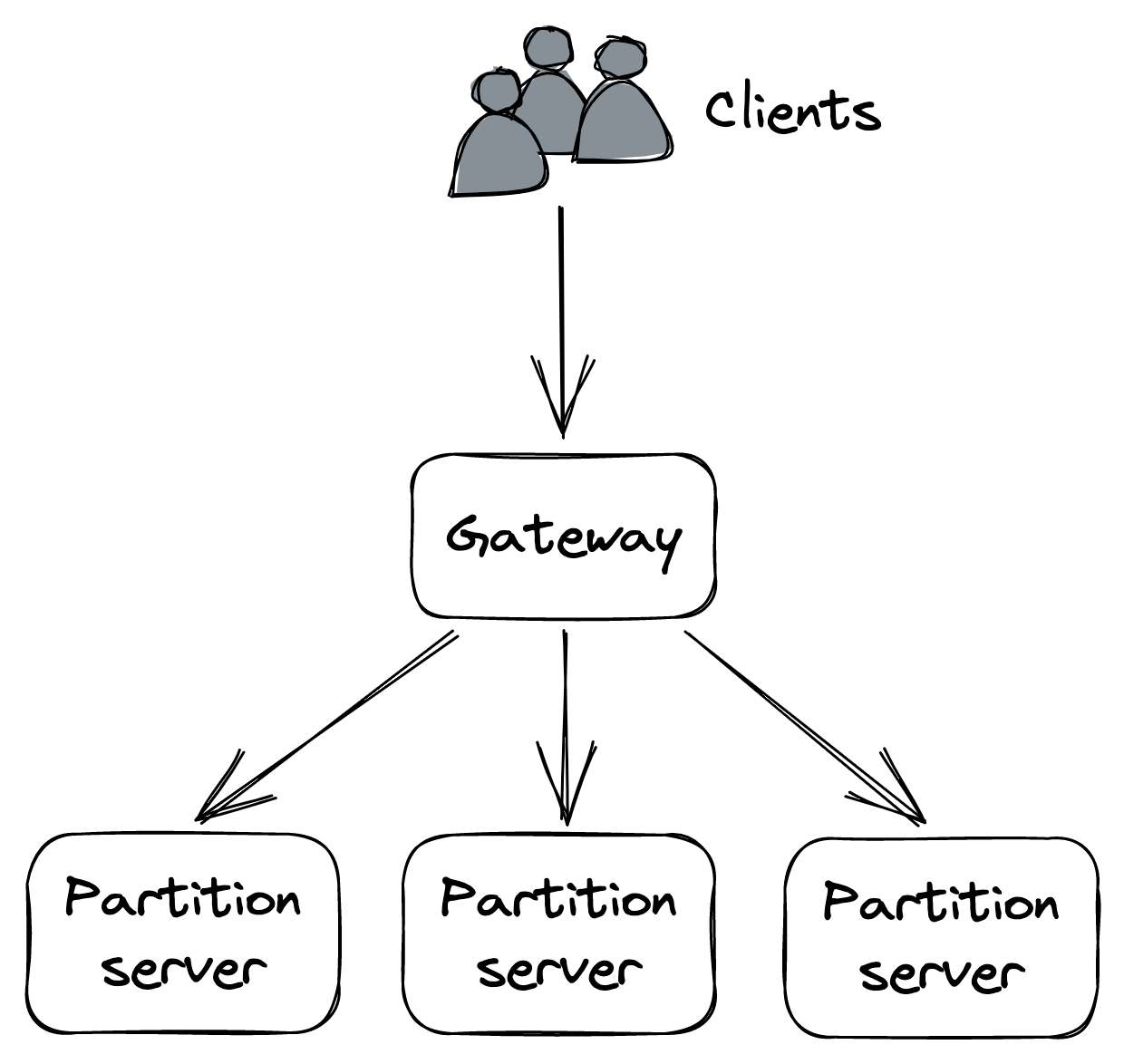
Figure 16.1: A partitioned application with a gateway that routes requests to partitions
- Transactions are required to atomically update data that spans multiple partitions, limiting scalability.
- If a partition is accessed much more frequently than others, the system’s ability to scale is limited.
- Adding or removing partitions at run time becomes challenging, since it requires moving data across nodes.
It’s no coincidence we are talking about partitioning right after discussing CDNs. A cache lends itself well to partitioning as it avoids most of this complexity. For example, it generally doesn’t need to atomically update data across partitions or perform aggregations spanning multiple partitions.
Now that we have an idea of what partitioning is and why it’s useful, let’s discuss how data, in the form of key-value pairs, can be mapped to partitions. At a high level, there are two main ways of doing that, referred to as range partitioning and hash partitioning. An important prerequisite for both is that the number of possible keys is very large; for example, a boolean key with only two possible values is not suited for partitioning since it allows for at most two partitions.
Range partitioning
Range partitioning splits the data by key range into lexicographically sorted partitions, as shown in Figure 16.2. To make range scans fast, each partition is generally stored in sorted order on disk.
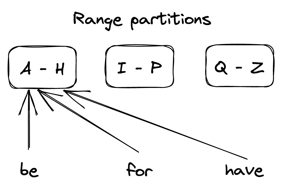
Figure 16.2: A range-partitioned dataset
The first challenge with range partitioning is picking the partition boundaries. For example, splitting the key range evenly makes sense if the distribution of keys is more or less uniform. If not, like in the English dictionary, the partitions will be unbalanced and some will have a lot more entries than others.
Another issue is that some access patterns can lead to hotspots, which affect performance. For example, if the data is range partitioned by date, all requests for the current day will be served by a single node. There are ways around that, like adding a random prefix to the partition keys, but there is a price to pay in terms of increased complexity.
When the size of the data or the number of requests becomes too large, the number of nodes needs to be increased to sustain the increase in load. Similarly, if the data shrinks and/or the number of requests drops, the number of nodes should be reduced to decrease costs. The process of adding and removing nodes to balance the system’s load is called rebalancing. Rebalancing has to be implemented in a way that minimizes disruption to the system, which needs to continue to serve requests. Hence, the amount of data transferred when rebalancing partitions should be minimized.
One solution is to create a lot more partitions than necessary when the system is first initialized and assign multiple partitions to each node. This approach is also called static partitioning since the number of partitions doesn’t change over time. When a new node joins, some partitions move from the existing nodes to the new one so that the store is always in a balanced state. The drawback of this approach is that the number of partitions is fixed and can’t be easily changed. Getting the number of partitions right is hard — too many partitions add overhead and decrease performance, while too few partitions limit scalability. Also, some partitions might end up being accessed much more than others, creating hotspots.
The alternative is to create partitions on demand, also referred to as dynamic partitioning. The system starts with a single partition, and when it grows above a certain size or becomes too hot, the partition is split into two sub-partitions, each containing approximately half of the data, and one of the sub-partitions is transferred to a new node. Similarly, when two adjacent partitions become small or “cold” enough, they can be merged into a single one.
Hash partitioning
Let’s take a look at an alternative way of mapping data to partitions. The idea is to use a hash function that deterministically maps a key (string) to a seemingly random number (a hash) within a certain range (e.g., 0 and 264 −1). This guarantees that the keys’ hashes are distributed uniformly across the range.
Next, we assign a subset of the hashes to each partition, as shown in Figure 16.3. For example, one way of doing that is by taking the modulo of a hash, i.e., hash(key) mod N, where N is the number of partitions.
Although this approach ensures that the partitions contain more
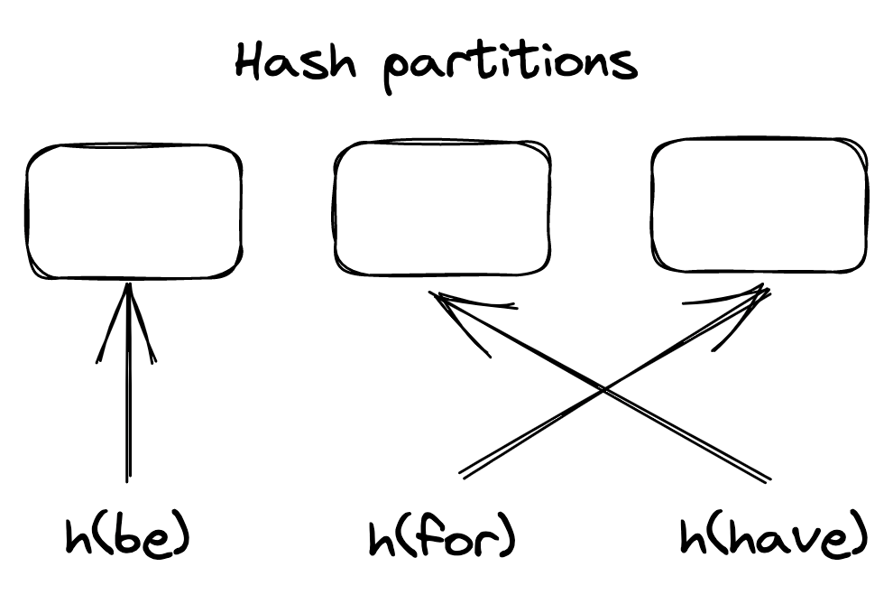
Figure 16.3: A hash-partitioned dataset
or less the same number of entries, it doesn’t eliminate hotspots if the access pattern is not uniform. For example, if a single key is accessed significantly more often than others, the node hosting the partition it belongs to could become overloaded. In this case, the partition needs to be split further by increasing the total number of partitions. Alternatively, the key needs to be split into sub-keys by, e.g., prepending a random prefix.
Assigning hashes to partitions via the modulo operator can become problematic when a new partition is added, as most keys have to be moved (or shuffled) to a different partition because their assignment changed. Shuffling data is extremely expensive as it consumes network bandwidth and other resources. Ideally, if a partition is added, only K
Nkeys should be shuffled around, where Kis the number of keys and Nis the number of partitions. One widely used hashing strategy with that property is consistent hashing.
With consistent hashing[1], a hash function randomly maps both the partition identifiers and keys onto a circle, and each key is assigned to the closest partition that appears on the circle in clockwise order (see Figure 16.4).
Now, when a new partition is added, only the keys that now map
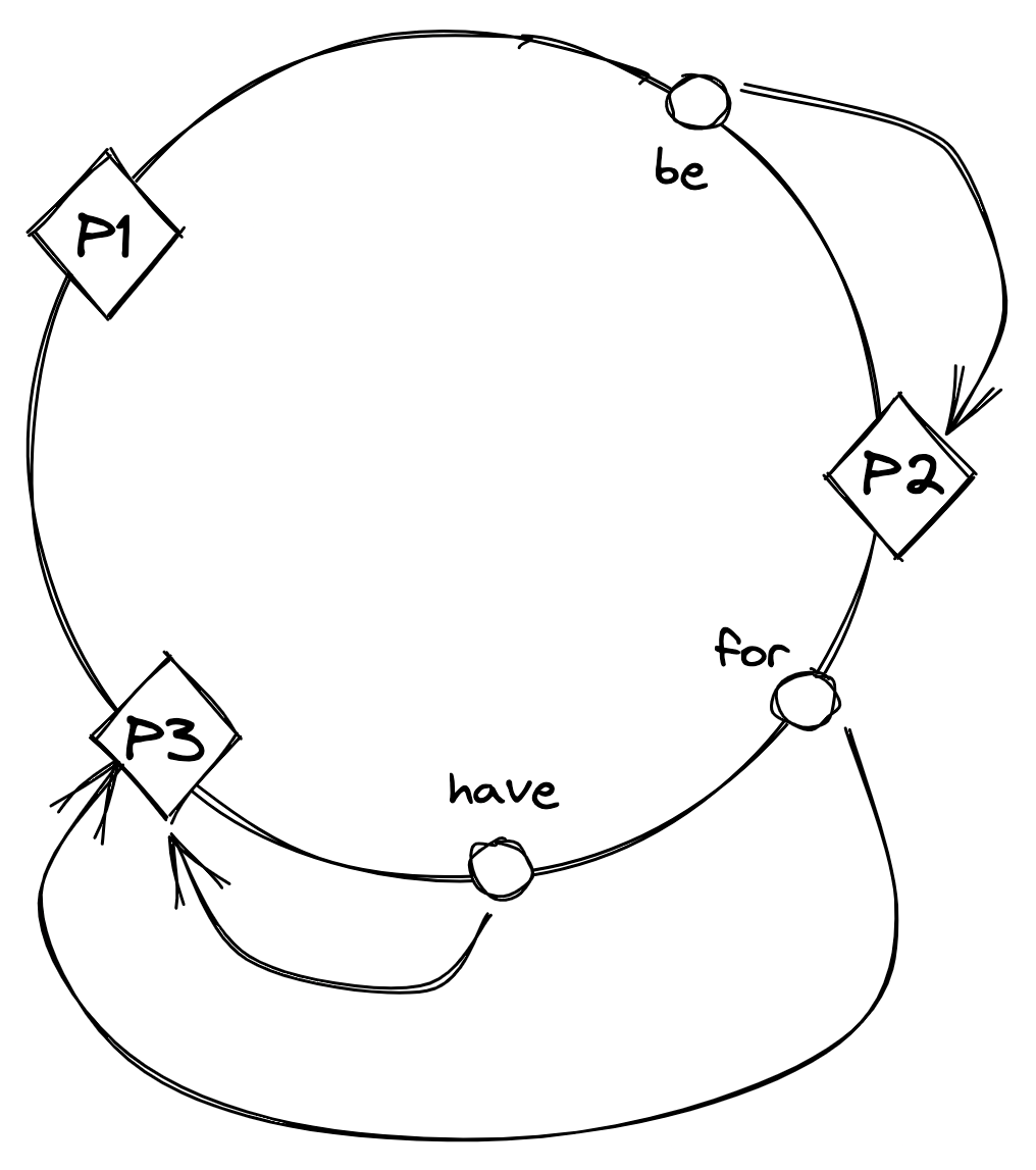
Figure 16.4: With consistent hashing, partition identifiers and keys are randomly distributed around a circle, and each key is assigned to the next partition that appears on the circle in clockwise order.
to it on the circle need to be reassigned, as shown in Figure 16.5.
The main drawback of hash partitioning compared to range partitioning is that the sort order over the partitions is lost, which is required to efficiently scan all the data in order. However, the data within an individual partition can still be sorted based on a secondary key.
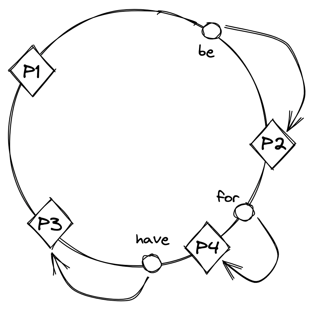
Figure 16.5: After partition P4 is added, the key ’for’ is reassigned to P4, but the assignment of the other keys doesn’t change.
File storage
Video coming soon. Start with the reading below.
Using a CDN has significantly reduced the number of requests hitting Cruder’s application server. But there are only so many images, videos, etc., the server can store on its local disk(s) before running out of space. To work around this limit, we can use a managed file store, like AWS S3[1] or Azure Blob Storage[2], to store large static files. Managed file stores are scalable, highly available, and offer strong durability guarantees. A file uploaded to a managed store can be configured to allow access to anyone who knows its URL, which means we can point the CDN straight at it. This allows us to completely offload the storage and serving of static resources to managed services.
Blob storage architecture
Because distributed file stores are such a crucial component of modern applications, it’s useful to have an idea of how they work underneath. In this lesson, we will dive into the architecture of
Azure Storage[3] (AS), a scalable cloud storage system that provides strong consistency. AS supports file, queue, and table abstractions, but for simplicity, our discussion will focus exclusively on the file abstraction, also referred to as the blob store.
AS is composed of storage clusters distributed across multiple regions worldwide. A storage cluster is composed of multiple racks of nodes, where each rack is built out as a separate unit with redundant networking and power.
At a high level, AS exposes a global namespace based on domain names that are composed of two parts: an account name and a file name. The two names together form a unique URL that points to a specific file, e.g., https://ACCOUNT_NAME.blob.core.windows.net/FILE_NAME . The customer configures the account name, and the AS DNS server uses it to identify the storage cluster where the data is stored. The cluster uses the file name to locate the node responsible for the data.
A central location service acts as the global control plane in charge of creating new accounts and allocating them to clusters, and also moving them from one cluster to another for better load distribution. For example, when a customer wants to create a new account in a specific region, the location service:
- chooses a suitable cluster to which to allocate the account based on load information;
- updates the configuration of the cluster to start accepting requests for the new account;
- and creates a new DNS record that maps the account name to the cluster’s public IP address.
From an architectural point of view, a storage cluster is composed of three layers: a stream layer, a partition layer, and a front-end layer (see Figure 17.1).
The stream layer implements a distributed append-only file system in which the data is stored in so-called streams. Internally, a stream
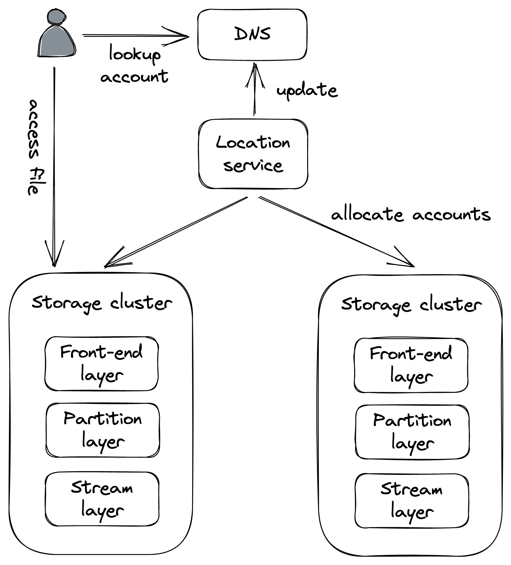
Figure 17.1: A high-level view of Azure Storage’s architecture
is represented as a sequence of extents, where the extent is the unit of replication. Writes to extents are replicated synchronously using chain replication[4].
The stream manager is the control plane responsible for assigning an extent to a chain of storage servers in the cluster. When the manager is asked to allocate a new extent, it replies with the list of storage servers that hold a copy of the newly created extent (see Figure 17.2). The client caches this information and uses it to send future writes to the primary server. The stream manager is also responsible for handling unavailable or faulty extent replicas by creating new ones and reconfiguring the replication chains they are part of.
The partition layer is where high-level file operations are translated
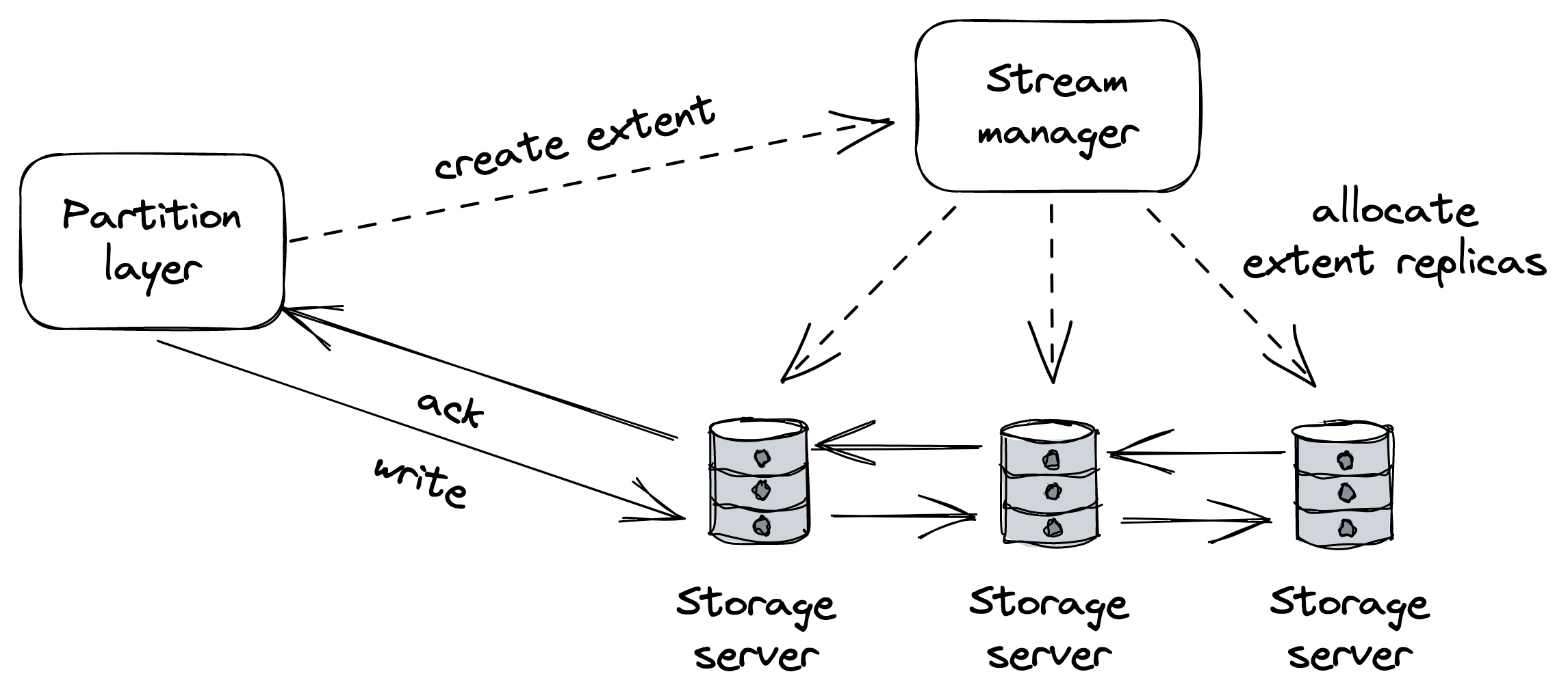
Figure 17.2: The stream layer uses chain replication to replicate extents across storage servers.
to low-level stream operations. Within this layer, the partition manager (yet another control plane) manages a large index of all files stored in the cluster. Each entry in the index contains metadata such as account and file name and a pointer to the actual data in the stream service (list of extent plus offset and length). The partition manager range-partitions the index and maps each partition to a partition server. The partition manager is also responsible for load-balancing partitions across servers, splitting partitions when they become too hot, and merging cold ones (see Figure 17.3).
The partition layer also asynchronously replicates accounts across clusters in the background. This functionality is used to migrate accounts from one cluster to another for load-balancing purposes and disaster recovery.
Finally, the front-end service (a reverse proxy) is a stateless service that authenticates requests and routes them to the appropriate partition server using the mapping managed by the partition manager.
Although we have only coarsely described the architecture of AS, it’s a great showcase of the scalability patterns applied to a concrete system. As an interesting historical note, AS was built from the ground up to be strongly consistent, while AWS S3 started of-
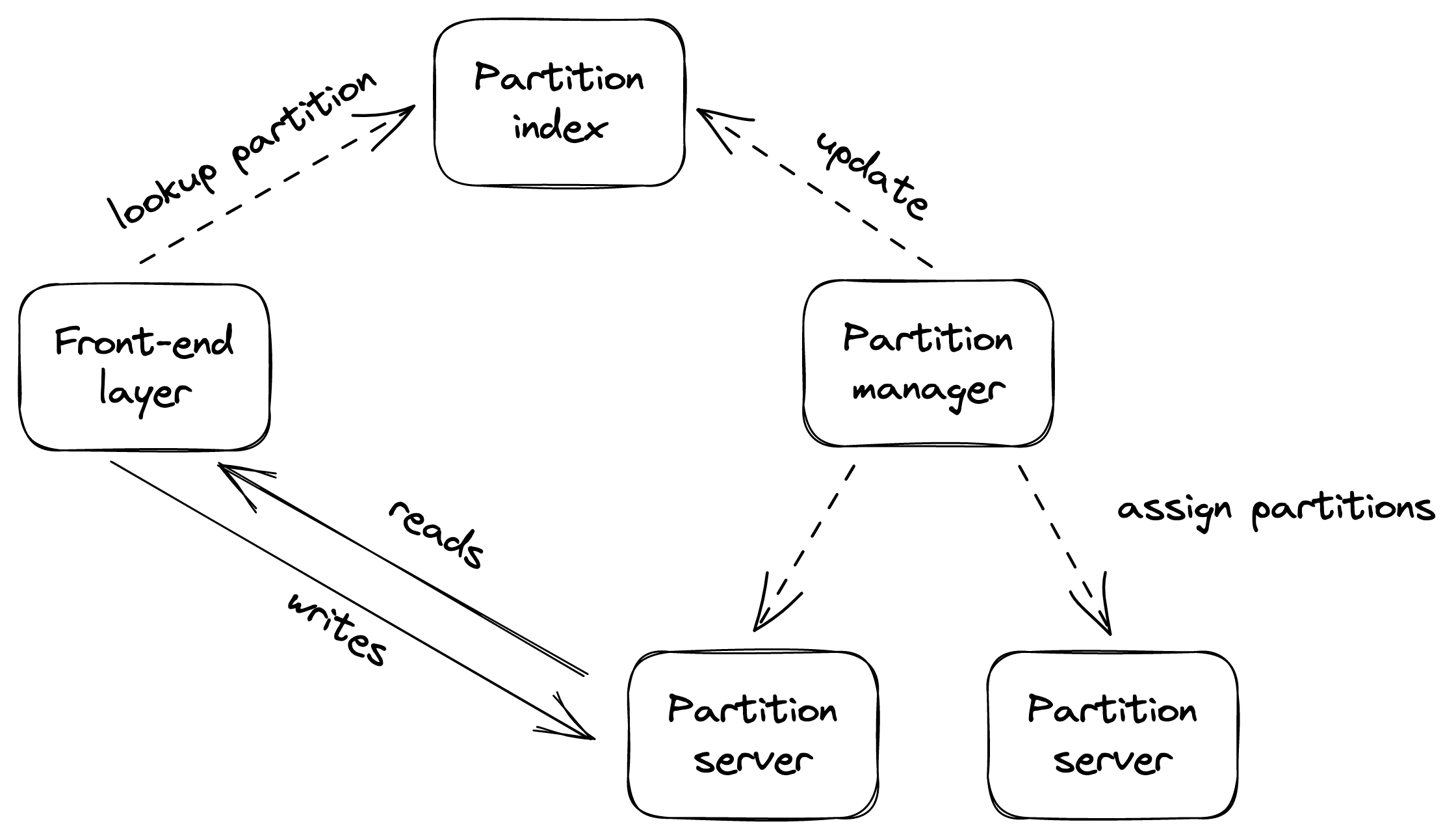
Figure 17.3: The partition manager range-partitions files across partition servers and rebalances the partitions when necessary.
fering the same guarantee in 2021[5].
Network load balancing
Video coming soon. Start with the reading below.
By offloading requests to the file store and the CDN, Cruder is able to serve significantly more requests than before. But the free lunch is only going to last so long. Because there is a single application server, it will inevitably fall over if the number of requests directed at it keeps increasing. To avoid that, we can create multiple application servers, each running on a different machine, and have a load balancer distribute requests to them. The thinking is that if one server has a certain capacity, then, in theory, two servers should have twice that capacity. This is an example of the more general scalability pattern we referred to as scaling out or scaling horizontally.
The reason we can scale Cruder horizontally is that we have pushed the state to dedicated services (the database and the managed file store). Scaling out a stateless application doesn’t require much effort, assuming its dependencies can scale accordingly as well. As we will discuss in Data storage (lesson 04.07), scaling out a stateful service, like a data store, is a lot more challenging since it needs to replicate state and thus requires some form of coordination, which adds complexity and can also become a bottleneck. As a general rule of thumb, we should try to keep our applications stateless by pushing state to third-party services designed by teams with years of experience building such services.
Distributing requests across a pool of servers has many benefits. Because clients are decoupled from servers and don’t need to know their individual addresses, the number of servers behind the load balancer can increase or decrease transparently. And since multiple redundant servers can interchangeably be used to handle requests, a load balancer can detect faulty ones and take them out of the pool, increasing the availability of the overall application.
As you might recall from Introduction (lesson 01.01), the availability of a system is the percentage of time it’s capable of servicing requests and doing useful work. Another way of thinking about it is that it’s the probability that a request will succeed.
The reason why a load balancer increases the theoretical availability is that in order for the application to be considered unavailable, all the servers need to be down. With N servers, the probability that they are all unavailable is the product of the servers’ failure rates[1]. By subtracting this product from 1, we can determine the theoretical availability of the application.
For example, if we have two servers behind a load balancer and each has an availability of 99%, then the application has a theoretical availability of 99.99%:
1 −(0.01 ⋅0.01) = 0.9999
Intuitively, the nines of independent servers sum up.[2] Thus, in the previous example, we have two independent servers with two nines each, for a total of four nines of availability. Of course, this number is only theoretical because, in practice, the load balancer doesn’t remove faulty servers from the pool immediately. The formula also naively assumes that the failure rates are independent, which might not be the case. Case in point: when a faulty server is removed from the load balancer’s pool, the remaining ones might not be able to sustain the increase in load and degrade.
In the following sections, we will take a closer look at some of the core features offered by a load balancer.
Load balancing
The algorithms used for routing requests can vary from roundrobin to consistent hashing to ones that take into account the servers’ load.
As a fascinating side note, balancing by load is a lot more challenging than it seems in a distributed context. For example, the load balancer could periodically sample a dedicated load endpoint exposed by each server that returns a measure of how busy the server is (e.g., CPU usage). And since constantly querying servers can be costly, the load balancer can cache the responses for some time.
Using cached or otherwise delayed metrics to distribute requests to servers can result in surprising behaviors. For example, if a server that just joined the pool reports a load of 0, the load balancer will hammer it until the next time its load is sampled. When that happens, the server will report that it’s overloaded, and the load balancer will stop sending more requests to it. This causes the server to alternate between being very busy and not being busy at all.
As it turns out, randomly distributing requests to servers without accounting for their load achieves a better load distribution. Does that mean that load balancing using delayed load metrics is not possible? There is a way, but it requires combining load metrics with the power of randomness. The idea is to randomly pick two servers from the pool and route the request to the least-loaded one of the two. This approach works remarkably well in practice[3].
Service discovery
Service discovery is the mechanism the load balancer uses to discover the pool of servers it can route requests to. A naive way to implement it is to use a static configuration file that lists the IP ad-dresses of all the servers, which is painful to manage and keep up to date.
A more flexible solution is to have a fault-tolerant coordination service, like, e.g., etcd or Zookeeper, manage the list of servers. When a new server comes online, it registers itself to the coordination service with a TTL. When the server unregisters itself, or the TTL expires because it hasn’t renewed its registration, the server is removed from the pool.
Adding and removing servers dynamically from the load balancer’s pool is a key functionality cloud providers use to implement autoscaling[4], i.e., the ability to spin up and tear down servers based on load.
Health checks
A load balancer uses health checks to detect when a server can no longer serve requests and needs to be temporarily removed from the pool. There are fundamentally two categories of health checks: passive and active.
A passive health check is performed by the load balancer as it routes incoming requests to the servers downstream. If a server isn’t reachable, the request times out, or the server returns a non-retriable status code (e.g., 503), the load balancer can decide to take that server out of the pool.
Conversely, an active health check requires support from the downstream servers, which need to expose a dedicated health endpoint that the load balancer can query periodically to infer the server’s health. The endpoint returns 200 (OK) if the server can serve requests or a 5xx status code if it’s overloaded and doesn’t have more capacity to serve requests. If a request to the endpoint times out, it also counts as an error.
The endpoint’s handler could be as simple as always returning 200 OK, since most requests will time out when the server is degraded. Alternatively, the handler can try to infer whether the server is degraded by comparing local metrics, like CPU usage, available memory, or the number of concurrent requests being served, with configurable thresholds.
But here be dragons[5]: if a threshold is misconfigured or the health check has a bug, all the servers behind the load balancer may fail the health check. In that case, the load balancer could naively empty the pool, taking the application down. However, in practice, if the load balancer is “smart enough,” it should detect that a large fraction of the servers are unhealthy and consider the health checks to be unreliable. So rather than removing servers from the pool, it should ignore the health checks altogether so that new requests can be sent to any server.
Thanks to health checks, the application behind the load balancer can be updated to a new version without any downtime. During the update, a rolling number of servers report themselves as unavailable so that the load balancer stops sending requests to them. This allows in-flight requests to complete (drain) before the servers are restarted with the new version. More generally, we can use this mechanism to restart a server without causing harm.
For example, suppose a stateless application has a rare memory leak that causes a server’s available memory to decrease slowly over time. When the server has very little physical memory available, it will swap memory pages to disk aggressively. This constant swapping is expensive and degrades the performance of the server dramatically. Eventually, the leak will affect the majority of servers and cause the application to degrade.
In this case, we could force a severely degraded server to restart. That way, we don’t have to develop complex recovery logic when a server gets into a rare and unexpected degraded mode. Moreover, restarting the server allows the system to self-heal, giving its operators time to identify the root cause.
To implement this behavior, a server could have a separate background thread — a watchdog — that wakes up periodically and monitors the server’s health. For example, the watchdog could monitor the available physical memory left. When a monitored metric breaches a specific threshold for some time, the watchdog considers the server degraded and deliberately crashes or restarts it.
Of course, the watchdog’s implementation needs to be well-tested and monitored since a bug could cause servers to restart continuously. That said, I find it uncanny how this simple pattern can make an application a lot more robust to gray failures.
DNS load balancing
Now that we are familiar with the job description of a load balancer, let’s take a closer look at how it can be implemented. While you won’t have to build your own load balancer given the abundance of off-the-shelf solutions available, it’s important to have a basic knowledge of how a load balancer works. Because every request needs to go through it, it contributes to your applications’ performance and availability.
A simple way to implement a load balancer is with DNS. For example, suppose we have a couple of servers that we would like to load-balance requests over. If these servers have public IP ad-dresses, we can add those to the application’s DNS record and have the clients pick one[6] when resolving the DNS address, as shown in Figure 18.1.
Although this approach works, it’s not resilient to failures. If one of the two servers goes down, the DNS server will happily continue to serve its IP address, unaware that it’s no longer available. Even if we were to automatically reconfigure the DNS record when a failure happens and take out the problematic IP, the change needs
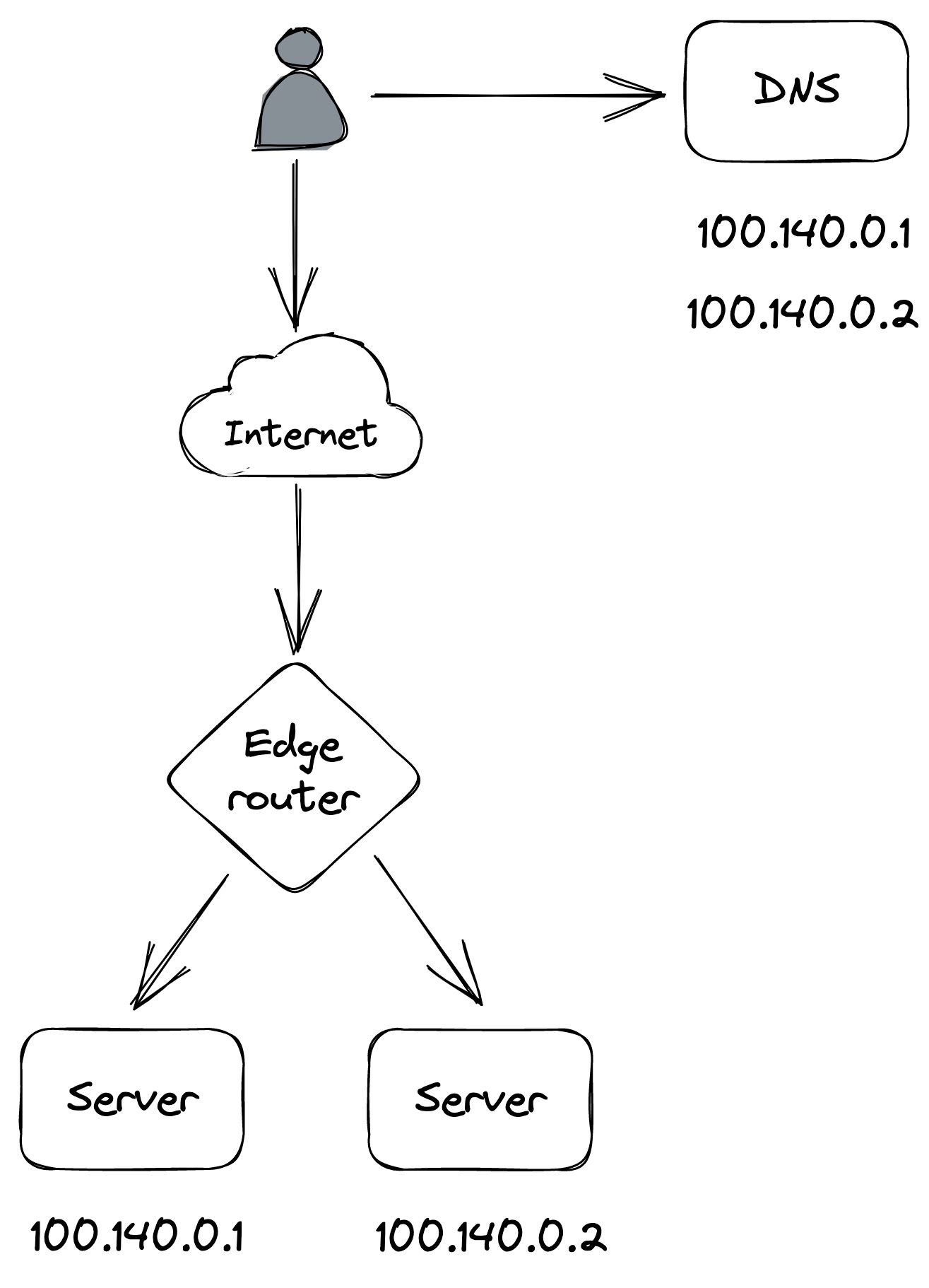
Figure 18.1: DNS load balancing
time to propagate to the clients, since DNS entries are cached, as discussed in Discovery (lesson 02.04).
The one use case where DNS is used in practice to load-balance is for distributing traffic to different data centers located in different regions (global DNS load balancing). We have already encountered a use for this when discussing CDNs.
Transport layer load balancing
A more flexible load-balancing solution can be implemented with a load balancer that operates at the TCP level of the network stack (aka L4 load balancer[7]) through which all the traffic between clients and servers flows.
A network load balancer has one or more physical network interface cards mapped to one or more virtual IP (VIP) addresses. A VIP, in turn, is associated with a pool of servers. The load balancer acts as an intermediary between clients and servers — clients only see the VIP exposed by the load balancer and have no visibility of the individual servers associated with it.
When a client creates a new TCP connection with a load balancer’s VIP, the load balancer picks a server from the pool and henceforth shuffles the packets back and forth for that connection between the client and the server. And because all the traffic goes through the load balancer, it can detect servers that are unavailable (e.g., with a passive health check) and automatically take them out of the pool, improving the system’s reliability.
A connection is identified by a tuple (source IP/port, destination IP/port). Typically, some form of hashing is used to assign a connection tuple to a server that minimizes the disruption caused by a server being added or removed from the pool, like consistent hashing[8].
To forward packets downstream, the load balancer translates[9] each packet’s source address to the load balancer’s address and its destination address to the server’s address. Similarly, when the load balancer receives a packet from the server, it translates its source address to the load balancer’s address and its destination address to the client’s address (see Figure 18.2).
As the data going out of the servers usually has a greater volume than the data coming in, there is a way for servers to bypass the load balancer and respond directly to the clients using a mechanism called direct server return[10], which can significantly reduce the load on the load balancer.
A network load balancer can be built using commodity machines
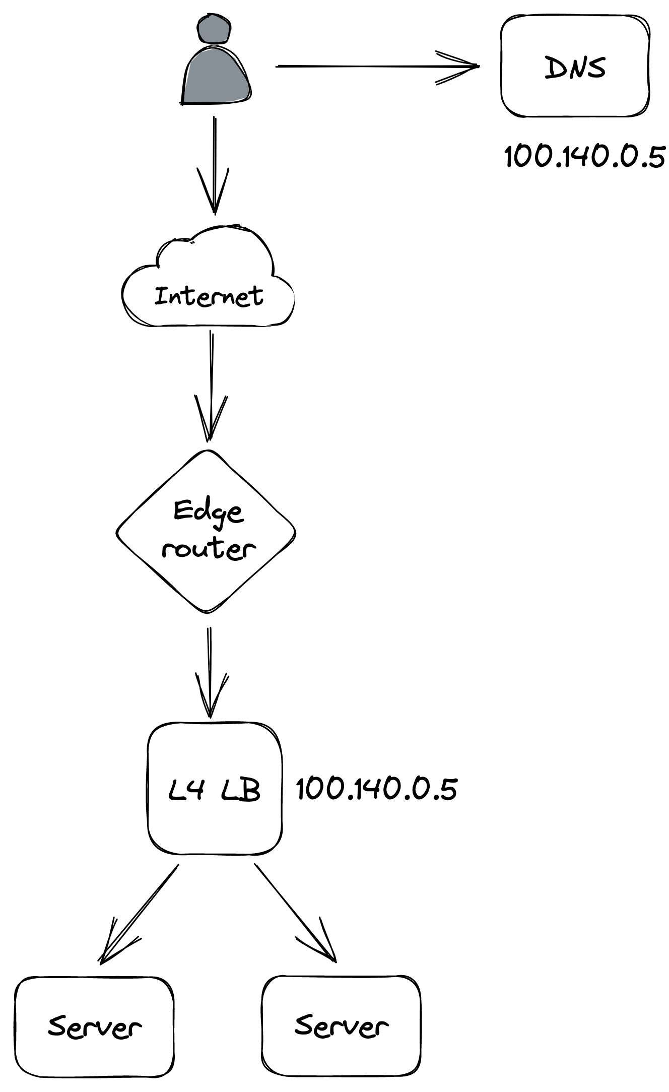
Figure 18.2: Transport layer load balancing
and scaled out using a combination of Anycast[11] and ECMP[12]. Load balancer instances announce themselves to the data center’s edge routers with the same Anycast VIP and identical BGP weight. Using an Anycast IP is a neat trick that allows multiple machines to share the same IP address and have routers send traffic to the one with the lowest BGP weight. If all the instances have the same identical BGP weight, routers use equal-cost multi-path routing (consistent hashing) to ensure that the packets of a specific connection are generally routed to the same load balancer instance.
Since Cruder is hosted in the cloud, we can leverage one of the many managed solutions for network load balancing, such as AWS Network Load Balancer[13] or Azure Load Balancer[14].
Although load balancing connections at the TCP level is very fast, the drawback is that the load balancer is just shuffling bytes around without knowing what they actually mean. Therefore, L4 load balancers generally don’t support features that require higher-level network protocols, like terminating TLS connections. A load balancer that operates at a higher level of the network stack is required to support these advanced use cases.
Application layer load balancing
An application layer load balancer (aka L7 load balancer[15]) is an HTTP reverse proxy that distributes requests over a pool of servers. The load balancer receives an HTTP request from a client, inspects it, and sends it to a backend server.
There are two different TCP connections at play here, one between the client and the L7 load balancer and another between the L7 load balancer and the server. Because a L7 load balancer operates at the HTTP level, it can de-multiplex individual HTTP requests sharing the same TCP connection. This is even more important with HTTP 2, where multiple concurrent streams are multiplexed on the same TCP connection, and some connections can be a lot more expensive to handle than others.
The load balancer can do smart things with application traffic, like rate-limit requests based on HTTP headers, terminate TLS connections, or force HTTP requests belonging to the same logical session to be routed to the same backend server. For example, the load balancer could use a cookie to identify which logical session a request belongs to and map it to a server using consistent hashing. That allows servers to cache session data in memory and avoid fetching it from the data store for each request. The caveat is that sticky sessions can create hotspots, since some sessions can be much more expensive to handle than others.
A L7 load balancer can be used as the backend of a L4 load balancer that load-balances requests received from the internet. Although L7 load balancers have more capabilities than L4 load balancers, they also have lower throughput, making L4 load balancers better suited to protect against certain DDoS attacks, like SYN floods[16].
A drawback of using a dedicated load balancer is that all the traffic directed to an application needs to go through it. So if the load balancer goes down, the application behind it does too. However, if the clients are internal to the organization, load balancing can be delegated to them using the sidecar pattern. The idea is to proxy all a client’s network traffic through a process co-located on the same machine (the sidecar proxy). The sidecar process acts as a L7 load balancer, load-balancing requests to the right servers. And, since it’s a reverse proxy, it can also implement various other functions, such as rate-limiting, authentication, and monitoring.
This approach[17] (aka “service mesh”) has been gaining popularity with the rise of microservices in organizations with hundreds of services communicating with each other. As of this writing, popular sidecar proxy load balancers are NGINX, HAProxy, and Envoy. The main advantage of this approach is that it delegates load-balancing to the clients, removing the need for a dedicated load balancer that needs to be scaled out and maintained. The drawback is that it makes the system a lot more complex since now we need a control plane to manage all the sidecars[18].
Data storage
Video coming soon. Start with the reading below.
Because Cruder is stateless, we were able to scale it out by running multiple application servers behind a load balancer. But as the application handles more load, the number of requests to the relational database increases as well. And since the database is hosted on a single machine, it’s only a matter of time until it reaches its capacity and it starts to degrade.
Replication
We can increase the read capacity of the database by creating replicas. The most common way of doing that is with a leader-follower topology (see Figure 19.1). In this model, clients send writes (updates, inserts, and deletes) exclusively to the leader, which persists the changes to its write-ahead log. Then, the followers, or replicas, connect to the leader and stream log entries from it, committing them locally. Since log entries have a sequence number, followers can disconnect and reconnect at any time and start from where they left off by communicating to the leader the last sequence number they processed.
By creating read-only followers and putting them behind a load balancer, we can increase the read capacity of the database. Repli-
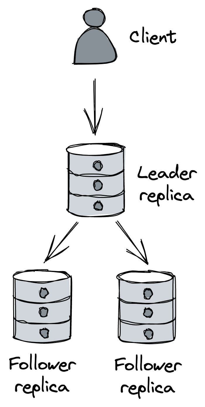
Figure 19.1: Single leader replication
cation also increases the availability of the database. For example, the load balancer can automatically take a faulty replica out of the pool when it detects that it’s no longer healthy or available. And when the leader fails, a replica can be reconfigured to take its place. Additionally, individual followers can be used to isolate specific workloads, like expensive analytics queries that are run periodically, so that they don’t impact the leader and other replicas.
The replication between the leader and the followers can happen either fully synchronously, fully asynchronously, or as a combination of the two.
If the replication is fully asynchronous, when the leader receives a write, it broadcasts it to the followers and immediately sends a response back to the client without waiting for the followers to acknowledge it. Although this approach minimizes the response time for the client, it’s not fault-tolerant. For example, the leader could crash right after acknowledging a write and before broadcasting it to the followers, resulting in data loss.
In contrast, if replication is fully synchronous, the leader waits for the write to be acknowledged by the followers before returning a response to the client. This comes with a performance cost since a single slow replica increases the response time of every request. And if any replica is unreachable, the data store becomes unavailable. This approach is not scalable; the more followers there are, the more likely it is that at least one of them is slow or unavailable.
In practice, relational databases often support a combination of synchronous and asynchronous replication. For example, in PostgreSQL, individual followers can be configured to receive updates synchronously[1], rather than asynchronously, which is the default. So, for example, we could have a single synchronous follower whose purpose is to act as an up-to-date backup of the leader. That way, if the leader fails, we can fail over to the synchronous follower without incurring any data loss.
Conceptually, the failover mechanism needs to: detect when the leader has failed, promote the synchronous follower to be the new leader and reconfigure the other replicas to follow it, and ensure client requests are sent to the new leader. Managed solutions like AWS RDS or Azure SQL Database, support read replicas[2] and automated failover[3] out of the box, among other features such as automated patching and backups.
One caveat of replication is that it only helps to scale out reads, not writes. The other issue is that the entire database needs to fit on a single machine. Although we can work around that by moving some tables from the main database to others running on different nodes, we would only be delaying the inevitable. As you should know by now, we can overcome these limitations with partitioning.
Partitioning
Partitioning allows us to scale out a database for both reads and writes. Even though traditional (centralized) relational databases generally don’t support it out of the box, we can implement it at the application layer in principle. However, implementing partitioning at the application layer is challenging and adds a lot of complexity to the system. For starters, we need to decide how to partition the data among the database instances and rebalance it when a partition becomes too hot or too big. Once the data is partitioned, queries that span multiple partitions need to be split into sub-queries and their responses have to be combined (think of aggregations or joins). Also, to support atomic transactions across partitions, we need to implement a distributed transaction protocol, like 2PC. Add to all that the requirement to combine partitioning with replication, and you can see how partitioning at the application layer becomes daunting.
Taking a step back, the fundamental problem with traditional relational databases is that they have been designed under the assumption they fit on a single beefy machine. Because of that, they support a number of features that are hard to scale, like ACID transactions and joins. Relational databases were designed in an era where disk space was costly, and normalizing the data to reduce the footprint on disk was a priority, even if it came with a significant cost to unnormalize the data at query time with joins.[4]
Times have changed, and storage is cheap nowadays, while CPU time isn’t. This is why, in the early 2000s, large tech companies began to build bespoke solutions for storing data designed from the ground up with high availability and scalability in mind.
NoSQL
These early solutions didn’t support SQL and more generally only implemented a fraction of the features offered by traditional relational data stores. White papers such as Bigtable[5] and Dynamo[6] revolutionized the industry and started a push towards scalable storage layers, resulting in a plethora of open source solutions inspired by them, like HBase and Cassandra.
Since the first generation of these data stores didn’t support SQL, they were referred to as NoSQL. Nowadays, the designation is misleading as NoSQL stores have evolved to support features, like dialects of SQL, that used to be available only in relational data stores.
While relational databases support stronger consistency models such as strict serializability, NoSQL stores embrace relaxed consistency models such as eventual and causal consistency to support high availability.
Additionally, NoSQL stores generally don’t provide joins and rely on the data, often represented as key-value pairs or documents (e.g., JSON), to be unnormalized. A pure key-value store maps an opaque sequence of bytes (key) to an opaque sequence of bytes (value). A document store maps a key to a (possibly hierarchical) document without a strictly enforced schema. The main difference from a key-value store is that documents are interpreted and indexed and therefore can be queried based on their internal structure.
Finally, since NoSQL stores natively support partitioning for scalability purposes, they have limited support for transactions. For example, Azure Cosmos DB currently only supports transactions scoped to individual partitions. On the other hand, since the data is stored in unnormalized form, there is less need for transactions or joins in the first place.
Although the data models used by NoSQL stores are generally not relational, we can still use them to model relational data. But if we take a NoSQL store and try to use it as a relational database, we will end up with the worst of both worlds. If used correctly, NoSQL can handle many of the use cases that a traditional relational database can[7], while being essentially scalable from day 1.[8]
The main requirement for using a NoSQL data store efficiently is to know the access patterns upfront and model the data accordingly; let’s see why that is so important. Take Amazon DynamoDB[9], for example; its main abstraction is a table that contains items. Each item can have different attributes, but it must have a primary key that uniquely identifies an item.
The primary key can consist of either a single attribute, the partition key, or of two attributes, the partition key and the sort key. As you might suspect, the partition key dictates how the data is partitioned and distributed across nodes, while the sort key defines how the data is sorted within a partition, which allows for efficient range queries.
DynamoDB creates three replicas for each partition and uses state machine replication to keep them in sync[10]. Writes are routed to the leader, and an acknowledgment is sent to the client when two out of three replicas have received the write. Reads can be either eventually consistent (pick any replica) or strongly consistent (query the leader). Confusingly enough, the architecture of DynamoDB is very different from the one presented in the Dynamo paper, which we discussed in Dynamo-style data stores in Coordination avoidance.
At a high level, DynamoDB’s API supports:
- CRUD operations on single items,
- querying multiple items that have the same partition key (optionally specifying conditions on the sort key),
- and scanning the entire table.
There are no join operations, by design, since they don’t scale well. But that doesn’t mean we should implement joins in the application. Instead, as we will see shortly, we should model our data so that joins aren’t needed in the first place.
The partition and sort key attributes are used to model the table’s access patterns. For example, suppose the most common access pattern is retrieving the list of orders for a specific customer sorted by date. In that case, it would make sense for the table to have the customer ID as the partition key, and the order creation date as the sort key:
| PartitionKey | SortKey | Attribute | Attribute |
|---|---|---|---|
| jonsnow | 2021 07 13 - - | OrderID:1452 | Status: Shipped |
| aryastark | 2021 07 20 - - | OrderID:5252 | Status: Placed |
| branstark | 2021 07 22 - - | OrderID:5260 | Status: Placed |
Now suppose that we also want the full name of the customer in the list of orders. While, in a relational database, a table contains only entities of a certain type (e.g., customer), in NoSQL, a table can contain entities of multiple types. Thus, we could store both customers and orders within the same table:
| PartitionKey | SortKey | Attribute | Attribute |
|---|---|---|---|
| jonsnow | 2021 07 13 - - | OrderID:1452 | Status: Shipped |
| jonsnow | jonsnow | FullName: JonSnow | Address: ... |
| aryastark | 2021 07 20 - - | OrderID:5252 | Status: Placed |
| aryastark | aryastark | FullName: AryaStark | Address: ... |
Because a customer and its orders have the same partition key, we can now issue a single query that retrieves all entities for the desired customer.
See what we just did? We have structured the table based on the access patterns so that queries won’t require any joins. Now think for a moment about how you would model the same data in normalized form in a relational database. You would probably have one table for orders and another for customers. And, to perform the same query, a join would be required at query time, which would be slower and harder to scale.
The previous example is very simple, and DynamoDB supports secondary indexes to model more complex access patterns — local secondary indexes allow for alternate sort keys in the same table, while global secondary indexes allow for different partition and sort keys, with the caveat that index updates are asynchronous and eventually consistent.
It’s a common misconception that NoSQL data stores are more flexible than relational databases because they can seamlessly scale without modeling the data upfront. Nothing is further from the truth — NoSQL requires a lot more attention to how the data is modeled. Because NoSQL stores are tightly coupled to the access patterns, they are a lot less flexible than relational databases.
If there is one concept you should take away from this lesson, it’s this: using a NoSQL data store requires identifying the access patterns upfront to model the data accordingly. If you want to learn how to do that, I recommend reading “The DynamoDB Book”[11], even if you plan to use a different NoSQL store.
As scalable data stores keep evolving, the latest trend is to combine the scalability of NoSQL with the ACID guarantees of relational databases. These new data stores are also referred to as NewSQL[12]. While NoSQL data stores prioritize availability over consistency in the face of network partitions, NewSQL stores prefer consistency. The argument behind NewSQL stores is that, with the right design, the reduction in availability caused by enforcing strong consistency is hardly noticeable[13] for many applications. That, combined with the fact that perfect 100% availability is not possible anyway (availability is defined in 9s), has spurred the drive to build storage systems that can scale but favor consistency over availability in the presence of network partitions. CockroachDB[14] and Spanner15 are well-known examples of NewSQL data stores.
Caching
Video coming soon. Start with the reading below.
Suppose a significant fraction of requests that Cruder sends to its data store consists of a small pool of frequently accessed entries. In that case, we can improve the application’s performance and reduce the load on the data store by introducing a cache. A cache is a high-speed storage layer that temporarily buffers responses from an origin, like a data store, so that future requests can be served directly from it. It only provides best-effort guarantees, since its state is disposable and can be rebuilt from the origin. We have already seen some applications of caching when discussing the DNS protocol or CDNs.
For a cache to be cost-effective, the proportion of requests that can be served directly from it (hit ratio) should be high. The hit ratio depends on several factors, such as the universe of cachable objects (the fewer, the better), the likelihood of accessing the same objects repeatedly (the higher, the better), and the size of the cache (the larger, the better).
As a general rule of thumb, the higher up in the call stack caching is used, the more resources can be saved downstream. This is why the first use case for caching we discussed was client-side HTTP caching. However, it’s worth pointing out that caching is an optimization, and you don’t have a scalable architecture if the origin, e.g., the data store in our case, can’t withstand the load without the cache fronting it. If the access pattern suddenly changes, leading to cache misses, or the cache becomes unavailable, you don’t want your application to fall over (but it’s okay for it to become slower).
Policies
When a cache miss occurs, the missing object has to be requested from the origin, which can happen in two ways:
- After getting an “object-not-found” error from the cache, the application requests the object from the origin and updates the cache. In this case, the cache is referred to as a side cache, and it’s typically treated as a key-value store by the application.
- Alternatively, the cache is inline, and it communicates directly with the origin, requesting the missing object on behalf of the application. In this case, the application only ever accesses the cache. We have already seen an example of an inline cache when discussing HTTP caching.
Because a cache has a limited capacity, one or more entries need to be evicted to make room for new ones when its capacity is reached. Which entry to remove depends on the eviction policy used by the cache and the objects’ access pattern. For example, one commonly used policy is to evict the least recently used (LRU) entry.
A cache can also have an expiration policy that dictates when an object should be evicted, e.g., a TTL. When an object has been in the cache for longer than its TTL, it expires and can safely be evicted. The longer the expiration time, the higher the hit ratio, but also the higher the likelihood of serving stale and inconsistent data.
The expiration doesn’t need to occur immediately, and it can be deferred to the next time the entry is requested. In fact, that might be preferable — if the origin (e.g., a data store) is temporarily unavailable, it’s more resilient to return an object with an expired TTL to the application rather than an error.
An expiry policy based on TTL is a workaround for cache invalidation, which is very hard to implement in practice[1]. For example, if you were to cache the result of a database query, every time any of the data touched by that query changes (which could span thousands of records or more), the cached result would need to be invalidated somehow.
Local cache
The simplest way to implement a cache is to co-locate it with the client. For example, the client could use a simple in-memory hash table or an embeddable key-value store, like RocksDB[2], to cache responses (see Figure 20.1).
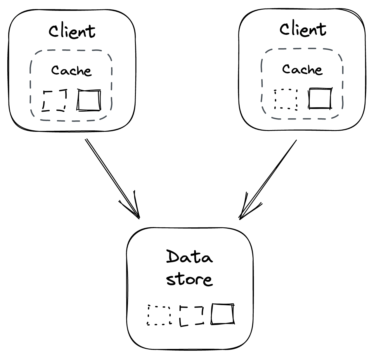
Figure 20.1: In-process cache
Because each client cache is independent of the others, the same objects are duplicated across caches, wasting resources. For example, if every client has a local cache of 1GB, then no matter how many clients there are, the total size of the cache is 1 GB. Also, consistency issues will inevitably arise; for example, two clients might see different versions of the same object.
Additionally, as the number of clients grows, the number of requests to the origin increases. This issue is exacerbated when clients restart, or new ones come online, and their caches need to be populated from scratch. This can cause a “thundering herd” effect where the downstream origin is hit with a spike of requests. The same can also happen when a specific object that wasn’t accessed before becomes popular all of a sudden.
Clients can reduce the impact of a thundering herd by coalescing requests for the same object. The idea is that, at any given time, there should be at most one outstanding request per client to fetch a specific object.
External cache
An external cache is a service dedicated to caching objects, typically in memory. Because it’s shared across clients, it addresses some of the drawbacks of local caches at the expense of greater complexity and cost (see Figure 20.2). For example, Redis[3] or Memcached[4] are popular caching services, also available as managed services on AWS and Azure.
Unlike a local cache, an external cache can increase its throughput and size using replication and partitioning. For example, Redis[5] can automatically partition data across multiple nodes and replicate each partition using a leader-follower protocol.
Since the cache is shared among its clients, there is only a single version of each object at any given time (assuming the cache is not replicated), which reduces consistency issues. Also, the number of times an object is requested from the origin doesn’t grow with the number of clients.
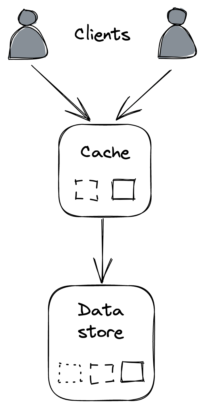
Figure 20.2: Out-of-process cache
Although an external cache decouples clients from the origin, the load merely shifts to the external cache. Therefore, the cache will eventually need to be scaled out if the load increases. When that happens, as little data as possible should be moved around (or dropped) to avoid the cache degrading or the hit ratio dropping significantly. Consistent hashing, or a similar partitioning technique, can help reduce the amount of data that needs to be shuffled when the cache is rebalanced.
An external cache also comes with a maintenance cost as it’s yet another service that needs to be operated. Additionally, the latency to access it is higher than accessing a local cache because a network call is required.
If the external cache is down, how should the clients react? You would think it might be okay to bypass the cache and directly hit the origin temporarily. But the origin might not be prepared to withstand a sudden surge of traffic. Consequently, the external cache becoming unavailable could cause a cascading failure, resulting in the origin becoming unavailable as well.
To avoid that, clients could use an in-process cache as a defense against the external cache becoming unavailable. That said, the origin also needs to be prepared to handle these sudden “attacks” by, e.g., shedding requests; we will discuss a few approaches for achieving that in this learning path’s resiliency part. What’s important to remember is that caching is an optimization, and the system needs to survive without it at the cost of being slower.
Microservices
Video coming soon. Start with the reading below.
If Cruder is successful in the market, we can safely assume that we will continue to add more components to it to satisfy an evergrowing list of business requirements, as shown in Figure 21.1.
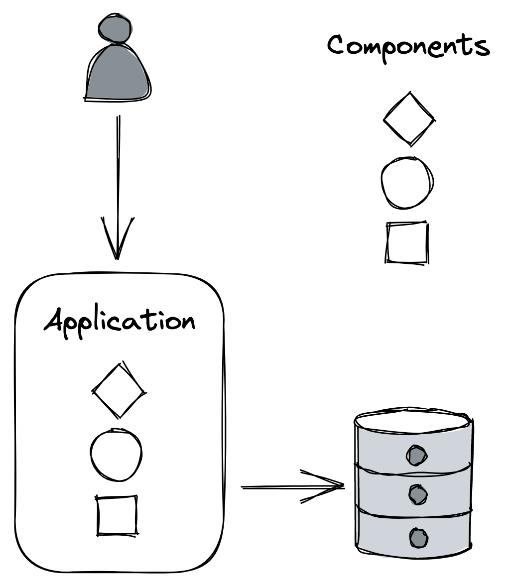
Figure 21.1: A monolithic application composed of multiple components
The components will likely become increasingly coupled in time, causing developers to step on each other’s toes more frequently. Eventually, the codebase becomes complex enough that nobody fully understands every part of it, and implementing new features or fixing bugs becomes a lot more time-consuming than it used to be.
Also, a change to a component might require the entire application to be rebuilt and deployed. And if the deployment of a new version introduces a bug, like a memory or socket leak, unrelated components might also be affected. Moreover, reverting a deployment affects the velocity of every developer, not just the one that introduced a bug.
One way to mitigate the growing pains of a monolithic application is to functionally decompose it into a set of independently deployable services that communicate via APIs, as shown in Figure 21.2. The APIs decouple the services from each other by creating boundaries that are hard to violate, unlike the ones between components running in the same process.
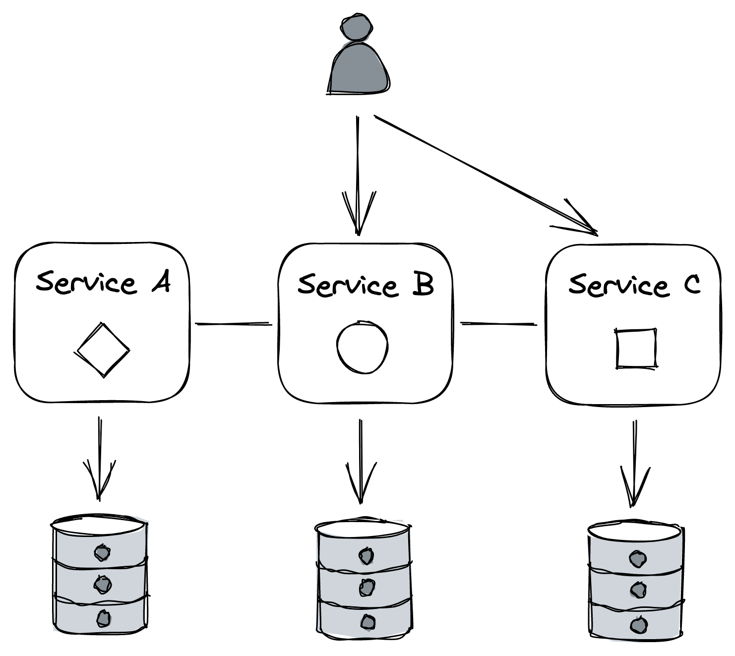
Figure 21.2: An application split into independently deployable services that communicate via APIs
Each service can be owned and operated by a small team. Smaller teams collaborate more effectively than larger ones, since the communication overhead grows quadratically[1] with the team’s size. And because each team controls its own codebase and dictates its own release schedule, less cross-team communication is required overall. Also, the surface area of a service is smaller than the whole application, making it more digestible to developers, especially new hires.
Each team is also free in principle to adopt the tech stack and hardware that fits their specific needs. After all, the consumers of the APIs don’t care how the functionality is implemented. This makes it easy to experiment and evaluate new technologies without affecting other parts of the system. As a result, each service can have its own independent data model and data store(s) that best fit its use cases.
This architectural style is also referred to as the microservice architecture. The term micro is misleading, though — there doesn’t have to be anything micro about services.[2] If a service doesn’t do much, it only adds operational overhead and complexity. As a rule of thumb, APIs should have a small surface area and encapsulate a significant amount of functionality.[3]
Caveats
To recap, splitting an application into services adds a great deal of complexity to the overall system, which is only worth paying if it can be amortized across many development teams. Let’s take a closer look at why that is.
Tech stack
While nothing forbids each microservice to use a different tech stack, doing so makes it more difficult for a developer to move from one team to another. And think of the sheer number of libraries — one for each language adopted — that need to be supported to provide common functionality that all services need, like logging.
It’s only reasonable, then, to enforce a certain degree of standardization. One way to do that, while still allowing some degree of freedom, is to loosely encourage specific technologies by providing a great development experience for the teams that stick with the recommended portfolio of languages and technologies.
Communication
Remote calls are expensive and introduce non-determinism. Much of what is described in this module is about dealing with the complexity of distributed processes communicating over the network. That said, a monolith doesn’t live in isolation either, since it serves external requests and likely depends on third-party APIs as well, so these issues need to be tackled there as well, albeit on a smaller scale.
Coupling
Microservices should be loosely coupled so that a change in one service doesn’t require changing others. When that’s not the case, you can end up with a dreaded distributed monolith, which has all the downsides of a monolith while being an order of magnitude more complex due to its distributed nature.
There are many causes of tight coupling, like fragile APIs that require clients to be updated whenever they change, shared libraries that have to be updated in lockstep across multiple services, or the use of static IP addresses to reference external services.
Resource provisioning
To support a large number of independent services, it should be simple to provision new machines, data stores, and other commodity resources — you don’t want every team to come up with their own way of doing it. And, once these resources have been provisioned, they have to be configured. To pull this off efficiently, a fair amount of automation is needed.
Testing
While testing individual microservices is not necessarily more challenging than testing a monolith, testing the integration of microservices is a lot harder. This is because very subtle and unexpected behaviors will emerge only when services interact with each other at scale in production.
Operations
Just like with resource provisioning, there should be a common way of continuously delivering and deploying new builds safely to production so that each team doesn’t have to reinvent the wheel.
Additionally, debugging failures, performance degradations, and bugs is a lot more challenging with microservices, as you can’t just load the whole application onto your local machine and step through it with a debugger. This is why having a good observability platform becomes crucial.
Eventual consistency
As a side effect of splitting an application into separate services, the data model no longer resides in a single data store. However, as we have learned in earlier lessons, atomically updating data spread in different data stores, and guaranteeing strong consistency, is slow, expensive, and hard to get right. Hence, this type of architecture usually requires embracing eventual consistency.
So to summarize, it’s generally best to start with a monolith and decompose it only when there is a good reason to do so[4]. As a bonus, you can still componentize the monolith, with the advantage that it’s much easier to move the boundaries as the application grows. Once the monolith is well matured and growing pains start to arise, you can start to peel off one microservice at a time from it.
API gateway
After decomposing Cruder into a group of services, we need to rethink how the outside world communicates with the application. For example, a client might need to perform multiple requests to different services to fetch all the information it needs to complete a specific operation. This can be expensive on mobile devices, where every network request consumes precious battery life.
Moreover, clients need to be aware of implementation details, such as the DNS names of all the internal services. This makes it challenging to change the application’s architecture as it requires changing the clients as well, which is hard to do if you don’t control them. Once a public API is out there, you had better be prepared to maintain it for a very long time.
As is common in computer science, we can solve almost any problem by adding a layer of indirection. We can hide the internal APIs behind a public one that acts as a facade, or proxy, for the internal services (see Figure 21.3). The service that exposes this public API is called the API gateway (a reverse proxy).
Core responsibilities
Let’s have a look at some of the most common responsibilities of an API gateway.
Routing
The most obvious function of an API gateway is routing inbound requests to internal services. One way to implement that is with the help of a routing map, which defines how the public API maps to the internal APIs. This mapping allows internal APIs to change without breaking external clients. For example, suppose there is a 1:1 mapping between a specific public endpoint and an internal one — if in the future the internal endpoint changes, the external clients can continue to use the public endpoint as if nothing had changed.
Composition
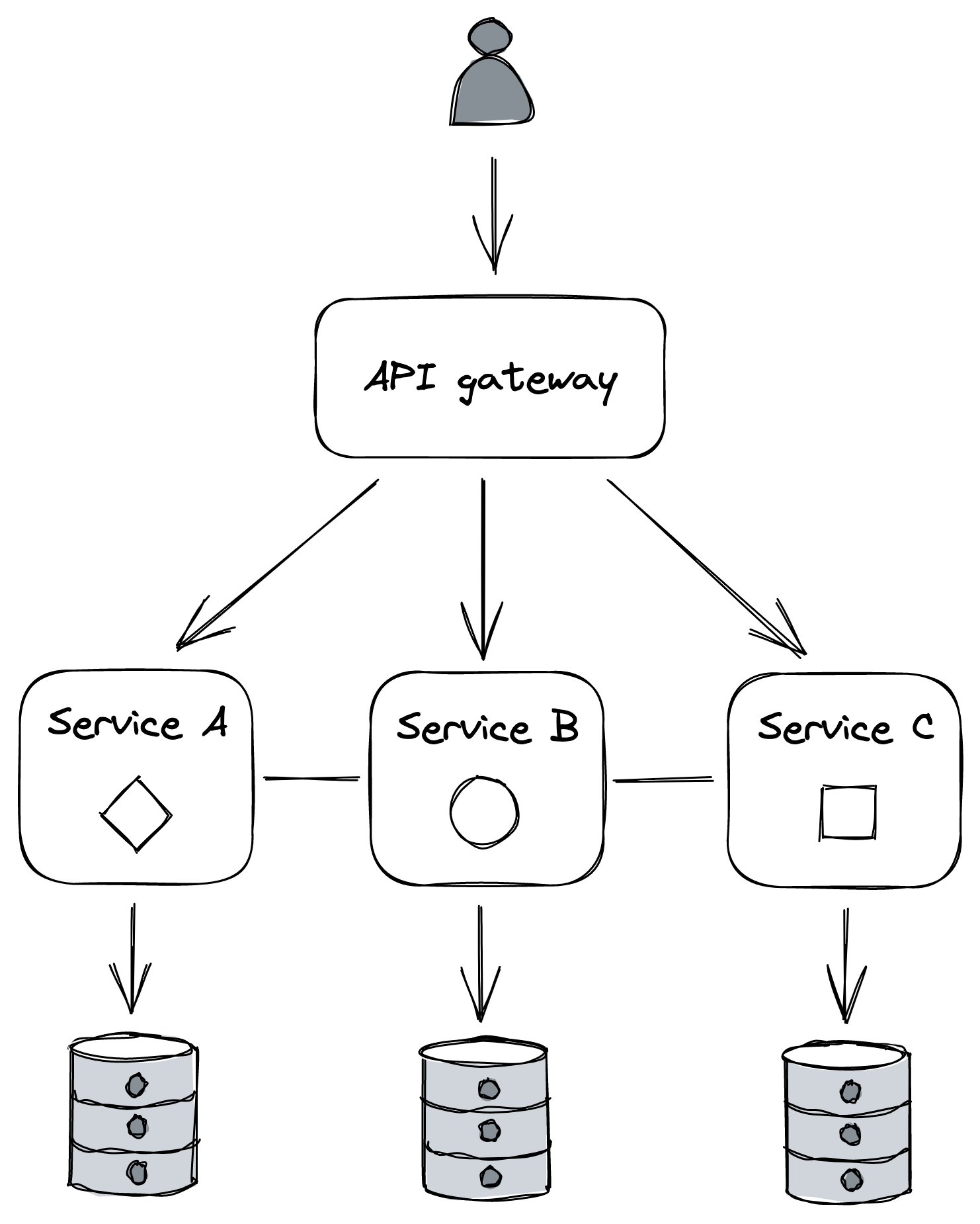
Figure 21.3: The API gateway hides the internal APIs from its clients.
The data of a monolithic application generally resides in a single data store, but in a distributed system, it’s spread across multiple services, each using its own data store. As such, we might encounter use cases that require stitching data together from multiple sources. The API gateway can offer a higher-level API that queries multiple services and composes their responses. This relieves the client from knowing which services to query and reduces the number of requests it needs to perform to get the data it needs.
Composing APIs is not simple. The availability of the composed API decreases as the number of internal calls increases, since each has a non-zero probability of failure. Moreover, the data might be inconsistent, as updates might not have propagated to all services yet; in that case, the gateway will have to resolve this discrepancy somehow.
Translation
The API gateway can translate from one IPC mechanism to another. For example, it can translate a RESTful HTTP request into an internal gRPC call.
It can also expose different APIs to different clients. For example, the API for a desktop application could potentially return more data than the one for a mobile application, as the screen estate is larger and more information can be presented at once. Also, network calls are more expensive for mobile clients, and requests generally need to be batched to reduce battery usage.
To meet these different and competing requirements, the gateway can provide different APIs tailored to different use cases and translate these to internal calls. Graph-based APIs are an increasingly popular solution for this. A graph-based API exposes a schema composed of types, fields, and relationships across types, which describes the data. Based on this schema, clients send queries declaring precisely what data they need, and the gateway’s job is to figure out how to translate these queries into internal API calls.
This approach reduces the development time as there is no need to introduce different APIs for different use cases, and clients are free to specify what they need. There is still an API, though; it just happens that it’s described with a graph schema, and the gateway allows to perform restricted queries on it. GraphQL[5] is the most popular technology in this space at the time of writing.
Cross-cutting concerns
As the API gateway is a reverse proxy, it can also implement cross-cutting functionality that otherwise would have to be part of each service. For example, it can cache frequently accessed resources or rate-limit requests to protect the internal services from being overwhelmed.
Authentication and authorization are some of the most common and critical cross-cutting concerns. Authentication is the process of validating that a so-called principal — a human or an application — issuing a request is who it says it is. Authorization is the process of granting the authenticated principal permissions to perform specific operations, like creating, reading, updating, or deleting a particular resource. Typically, this is implemented by assigning one or more roles that grant specific permissions to a principal.
A common way for a monolithic application to implement authentication and authorization is with sessions. Because HTTP is a stateless protocol, the application needs a way to store data between HTTP requests to associate a request with any other request. When a client first sends a request to the application, the application creates a session object with an ID (e.g., a cryptographicallystrong random number) and stores it in an in-memory cache or an external data store. The session ID is returned in the response through an HTTP cookie so that the client will include it in all future requests. That way, when the application receives a request with a session cookie, it can retrieve the corresponding session object.
So when a client sends its credentials to the application API’s login endpoint, and the credential validation is successful, the principal’s ID and roles are stored in the session object. The application can later retrieve this information and use it to decide whether to allow the principal to perform a request or not.
Translating this approach to a microservice architecture is not that straightforward. For example, it’s not obvious which service should be responsible for authenticating and authorizing requests, as the handling of requests can span multiple services.
One approach is to have the API gateway authenticate external requests, since that’s their point of entry. This allows centralizing the logic to support different authentication mechanisms into a single component, hiding the complexity from internal services. In contrast, authorizing requests is best left to individual services to avoid coupling the API gateway with domain logic.
When the API gateway has authenticated a request, it creates a security token. The gateway passes this token with the request to the internal services, which in turn pass it downstream to their dependencies. Now, when an internal service receives a request with a security token attached, it needs to have a way to validate it and obtain the principal’s identity and roles. The validation differs depending on the type of token used, which can be opaque and not contain any information, or transparent and embed the principal’s information within the token itself. The downside of an opaque token is that it requires calling an external auth service to validate it and retrieve the principal’s information. Transparent tokens eliminate that call at the expense of making it harder to revoke compromised tokens.
The most popular standard for transparent tokens is the JSON Web Token[6] (JWT). A JWT is a JSON payload that contains an expiration date, the principal’s identity and roles, and other metadata. In ad-dition, the payload is signed with a certificate trusted by the internal services. Hence, no external calls are needed to validate the token.
Another common mechanism for authentication is the use of API keys. An API key is a custom key that allows the API gateway to identify the principal making a request and limit what they can do. This approach is popular for public APIs, like the ones of, e.g., Github or Twitter.
We have barely scratched the surface of the topic, and there are entire books[7] written on the subject that you can read to learn more about it.
Caveats
One of the drawbacks of using an API gateway is that it can become a development bottleneck. Since it’s tightly coupled with the APIs of the internal services it’s shielding, whenever an internal
API changes, the gateway needs to be modified as well. Another downside is that it’s one more service that needs to be maintained. It also needs to scale to whatever the request rate is for all the services behind it.
That said, if an application has many services and APIs, the pros outweigh the cons, and it’s generally a worthwhile investment. So how do you go about implementing a gateway? You can roll your own API gateway, using a reverse proxy as a starting point, like NGINX, or use a managed solution, like Azure API Management[8] or Amazon API Gateway[9].
Control planes and data planes
Video coming soon. Start with the reading below.
The API gateway is a single point of failure. If it goes down, then so does Cruder, which is why it needs to be highly available. And because every external request needs to go through it, it must also be scalable. This creates some interesting challenges with regard to external dependencies.
For example, suppose the gateway has a specific “configuration” or management endpoint to add, remove and configure API keys used to rate-limit requests. Unsurprisingly, the request volume for the configuration endpoint is a lot lower than the one for the main endpoint(s), and a lower scale would suffice to handle it. And while the gateway needs to prefer availability and performance over consistency for routing external requests to internal services, it should prefer consistency over availability for requests sent to the management endpoint.
Because of these different and competing requirements, we could split the API gateway into a data plane service that serves external requests directed towards our internal services and a control plane service that manages the gateway’s metadata and configuration.
As it turns out, this split is a common pattern[1]. For example, in chain replication in Chain replication in Replication, the control plane holds the configuration of the chains. And in Azure Storage, which we discussed in File storage (lesson 04.05), the stream and partition managers are control planes that manage the allocation of streams and partitions to storage and partition servers, respectively.
More generally, a data plane includes any functionality on the critical path that needs to run for each client request. Therefore, it must be highly available, fast, and scale with the number of requests. In contrast, a control plane is not on the critical path and has less strict scaling requirements. Its main job is to help the data plane do its work by managing metadata or configuration and coordinating complex and infrequent operations. And since it generally needs to offer a consistent view of its state to the data plane, it favors consistency over availability.
An application can have multiple independent control and data planes. For example, a control plane might be in charge of scaling a service up or down based on load, while another manages its configuration.
But separating the control plane from the data plane introduces complexity. The data plane needs to be designed to withstand control plane failures for the separation to be robust. If the data plane stops serving requests when the control plane becomes unavailable, we say the former has a hard dependency on the latter. Intuitively, the entire system becomes unavailable if either the control plane or the data plane fails. More formally, when we have a chain of components that depend on each other, the theoretical availability of the system is the product of the availabilities of its components.
For example, if the data plane has a theoretical availability of 99.99%, but the control plane has an availability of 99%, then the overall system can only achieve a combined availability of 98.99%:
0.9999 ⋅0.99 = 0.9899
In other words, a system can at best be only as available as its least available hard dependency. We can try to make the control plane more reliable, but more importantly, we should ensure that the data plane can withstand control plane failures. If the control plane is temporarily unavailable, the data plane should continue to run with a stale configuration rather than stop. This concept is also referred to as static stability.
Scale imbalance
Generally, data planes and control planes tend to have very different scale requirements. This creates a risk as the data plane can overload[2] the control plane.
Suppose the control plane exposes an API that the data plane periodically queries to retrieve the latest configuration. Under normal circumstances, you would expect the requests to the control plane to be spread out in time more or less uniformly. But, in some cases, they can cluster within a short time interval. For example, if, for whatever reason, the processes that make up the data plane are restarted at the same time and must retrieve the configuration from the control plane, they could overload it.
Although the control plane can defend itself to some degree with the resiliency mechanisms described in Upstream resiliency (lesson 05.06), eventually, it will start to degrade. If the control plane becomes unavailable because of overload or any other reason (like a network partition), it can take down the data plane with it.
Going back to the previous example, if part of the data plane is trying to start but can’t reach the control plane because it’s overloaded, it won’t be able to come online. So how can we design around that?
One way is to use a scalable file store, like Azure Storage or S3, as a buffer between the control plane and the data plane. The control plane periodically dumps its entire state to the file store regardless of whether it changed, while the data plane reads the state periodically from it (see Figure 22.1). Although this approach sounds naive and expensive, it tends to be reliable and robust in practice. And, depending on the size of the state, it might be cheap too.[3]
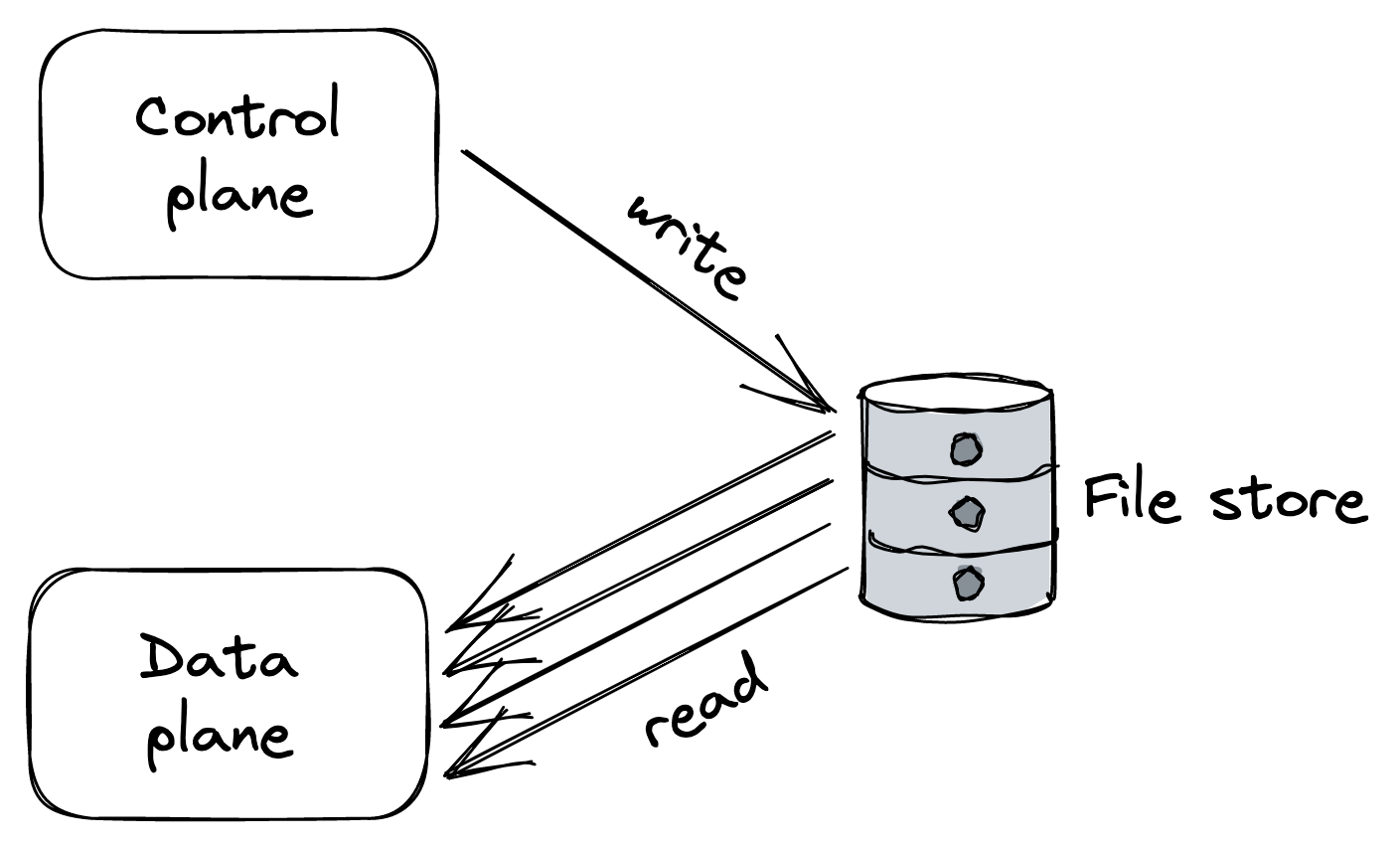
Figure 22.1: The intermediate data store protects the control plane by absorbing the load generated by the data plane.
Introducing an intermediate store as a buffer decouples the control plane from the data plane and protects the former from overload. It also enables the data plane to continue to operate (or start) if the control plane becomes unavailable. But this comes at the cost of higher latencies and weaker consistency guarantees, since the time it takes to propagate changes from the control plane to the data plane will necessarily increase.
To decrease the propagation latency, a different architecture is needed in which there is no intermediary. The idea is to have the data plane connect to the control plane, like in our original approach, but have the control plane push the configuration whenever it changes, rather than being at the mercy of periodic queries from the data plane. Because the control plane controls the pace, it will slow down rather than fall over when it can’t keep up.[4]
To further reduce latencies and load, the control plane can version changes and push only updates/deltas to the data plane. Although this approach is more complex to implement, it significantly reduces the propagation time when the state is very large.
However, the control plane could still get hammered if many data plane instances start up around the same time (due to a massive scale-out or restart) and try to read the entire configuration from the control plane for the first time. To defend against this, we can reintroduce an intermediate data store that contains a recent snapshot of the control plane’s state. This allows the data plane to read a snapshot from the store at startup and then request only a small delta from the control plane (see Figure 22.2).
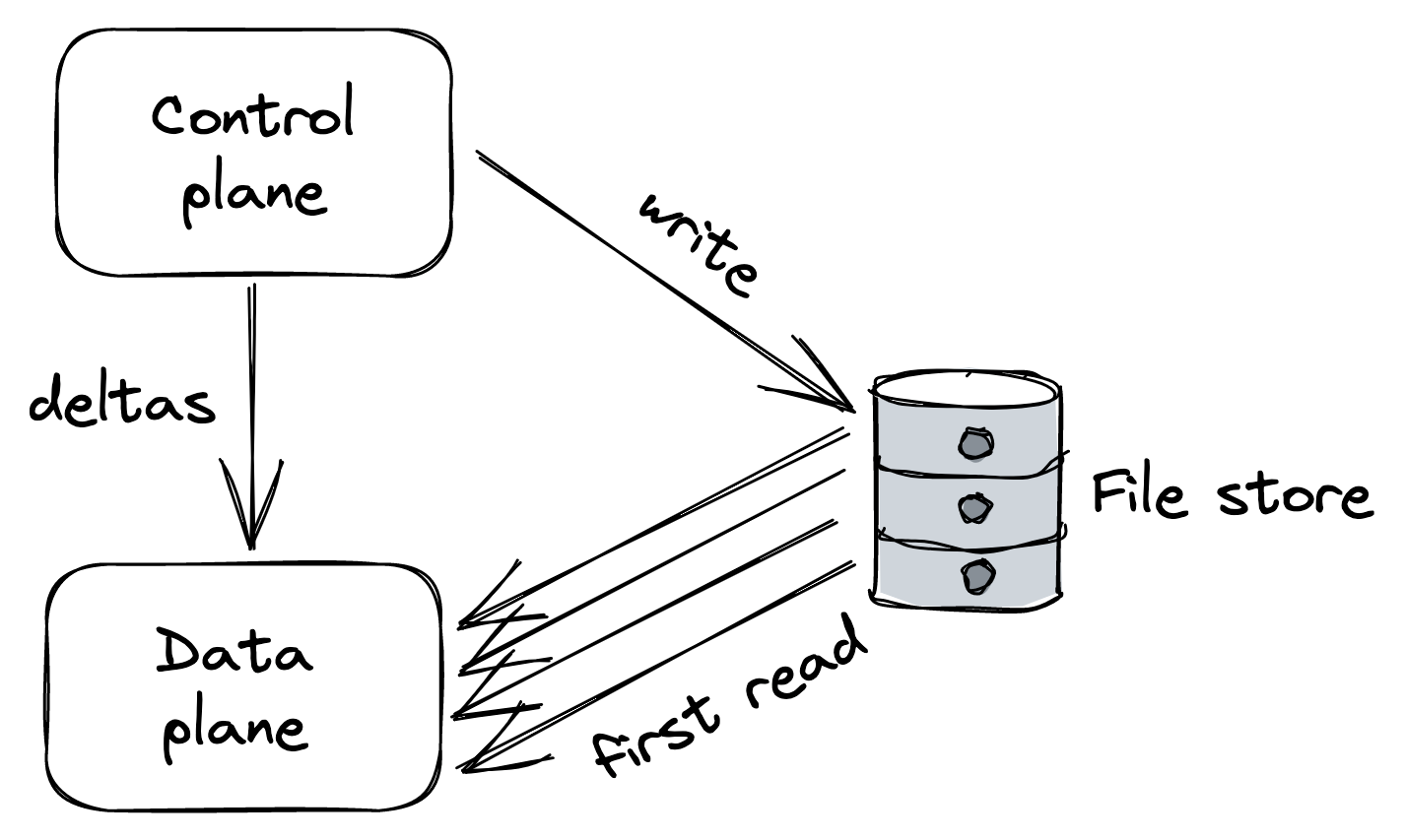
Figure 22.2: The intermediate data store absorbs the load of bulk reads, while the control plane pushes small deltas to the data plane whenever the state changes.
Control theory
Control theory gives us another[5] way to think about control planes and data planes. In control theory, the goal is to create a controller that monitors a dynamic system, compares its state to the desired one, and applies a corrective action to drive the system closer to it while minimizing any instabilities on the way.
In our case, the data plane is the dynamic system we would like to drive to the desired state, while the controller is the control plane responsible for monitoring the data plane, comparing it to the desired state, and executing a corrective action if needed.
The control plane and the data plane are part of a feedback loop. And without all three ingredients (monitor, compare, and action), you don’t have a closed loop, and the data plane can’t reach the desired state[6]. The monitoring part is the most commonly missing ingredient to achieve a closed loop.
Take chain replication, for example. The control plane’s job shouldn’t be just to push the configuration of the chains to the data plane. It should also monitor whether the data plane has actually applied the configuration within a reasonable time. If it hasn’t, it should perform some corrective action, which could be as naive as rebooting nodes with stale configurations or excluding them from being part of any chain.
A more mundane example of a control plane is a CI/CD pipeline for releasing a new version of a service without causing any disruption. One way to implement the pipeline is to deploy and release a new build blindly without monitoring the running service — the build might throw an exception at startup that prevents the service from starting, resulting in a catastrophic failure. Instead, the pipeline should release the new build incrementally while monitoring the service and stop the roll-out if there is clear evidence that something is off, and potentially also roll it back automatically.
To sum up, when dealing with a control plane, ask yourself what’s missing to close the loop. We have barely scratched the surface of the topic, and if you want to learn more about it, “Designing Distributed Control Systems”[7] is a great read.
Messaging
Video coming soon. Start with the reading below.
Suppose Cruder has an endpoint that allows users to upload a video and encode it in different formats and resolutions tailored to specific devices (TVs, mobile phones, tablets, etc.). When the API gateway receives a request from a client, it uploads the video to a file store, like S3, and sends a request to an encoding service to process the file.
Since the encoding can take minutes to complete, we would like the API gateway to send the request to the encoding service without waiting for the response. But the naive implementation (fireand-forget) would cause the request to be lost if the encoding service instance handling it on the other side crashes or fails for any reason.
A more robust solution is to introduce a message channel between the API gateway and the encoding service. Messaging was first introduced in APIs (lesson 02.05) when discussing APIs. It’s a form of indirect communication in which a producer writes a message to a channel — or message broker — that delivers the message to a consumer on the other end.
A message channel acts as a temporary buffer for the receiver. Unlike the direct request-response communication style we have been using so far, messaging is inherently asynchronous, as sending a message doesn’t require the receiving service to be online. The messages themselves have a well-defined format, consisting of a header and a body. The message header contains metadata, such as a unique message ID, while the body contains the actual content.
Typically, a message can either be a command, which specifies an operation to be invoked by the receiver, or an event, which signals the receiver that something of interest happened to the sender. A service can use inbound adapters to receive messages from channels and outbound adapters to send messages to channels, as shown in Figure 23.1.
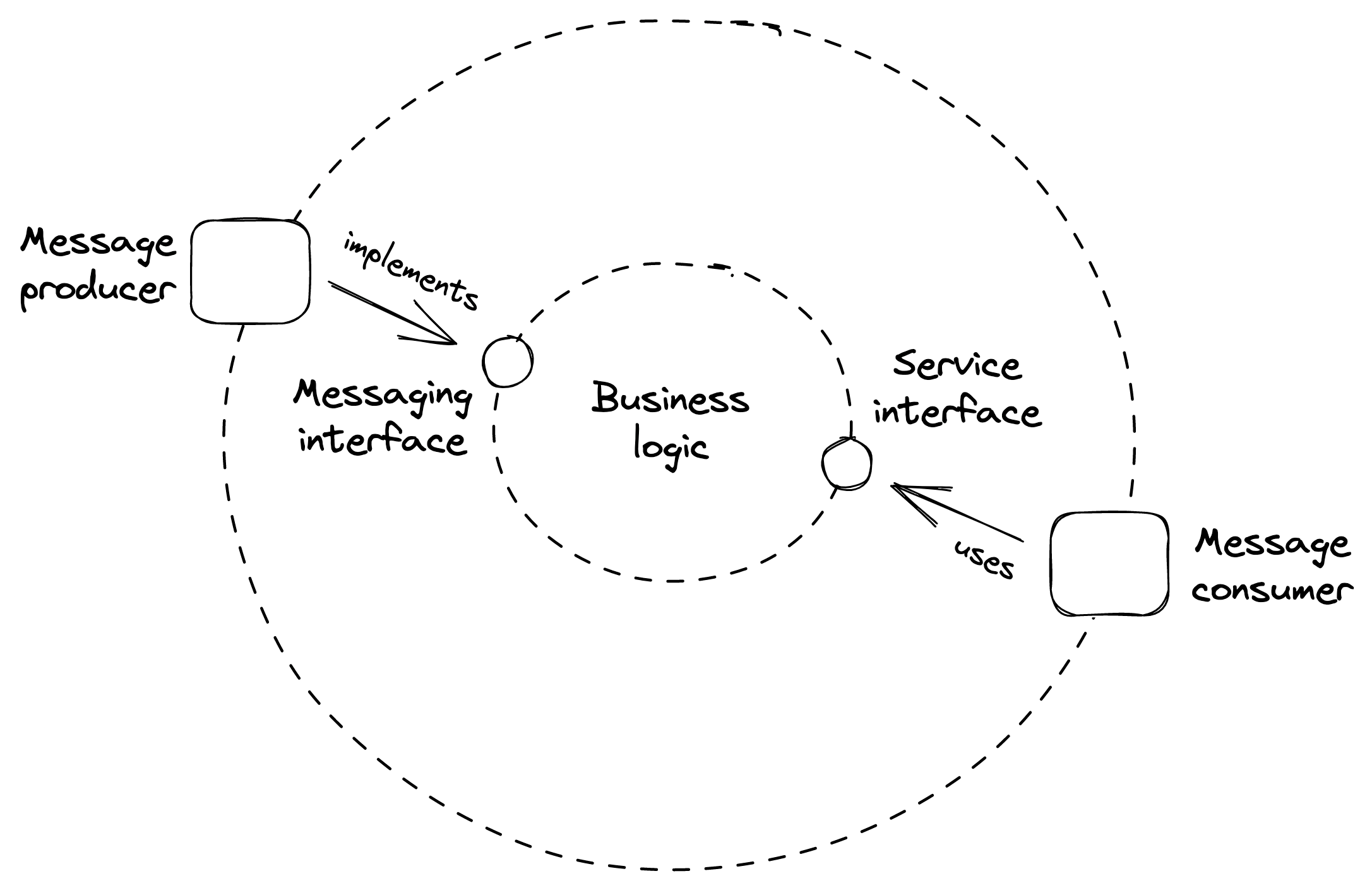
Figure 23.1: The message consumer (an inbound adapter) is part of the API surface of the service.
After the API gateway has uploaded the video to the file store, it writes a message to the channel with a link to the uploaded file and responds with 202 Accepted, signaling to the client that the request has been accepted for processing but hasn’t completed yet. Eventually, the encoding service will read the message from the channel and process it. Because the request is deleted from the channel only when it’s successfully processed, the request will eventually be picked up again and retried if the encoding service fails to handle it.
Decoupling the API gateway (producer) from the encoding service (consumer) with a channel provides many benefits. The producer can send requests to the consumer even if the consumer is temporarily unavailable. Also, requests can be load-balanced across a pool of consumer instances, making it easy to scale out the consuming side. And because the consumer can read from the channel at its own pace, the channel smooths out load spikes, preventing it from getting overloaded.
Another benefit is that messaging enables to process multiple messages within a single batch or unit of work. Most messaging brokers support this pattern by allowing clients to fetch up to N messages with a single read request. Although batching degrades the processing latency of individual messages, it dramatically improves the application’s throughput. So when we can afford the extra latency, batching is a no brainer.
In general, a message channel allows any number of producer and consumer instances to write and read from it. But depending on how the channel delivers a message, it’s classified as either pointto-point or publish-subscribe. In a point-to-point channel, the message is delivered to exactly one consumer instance. Instead, in a publish-subscribe channel, each consumer instance receives a copy of the message.
Unsurprisingly, introducing a message channel adds complexity. The message broker is yet another service that needs to be maintained and operated. And because there is an additional hop between the producer and consumer, the communication latency is necessarily going to be higher; more so if the channel has a large backlog of messages waiting to be processed. As always, it’s all about tradeoffs.
Because messaging is a core pattern of distributed systems, we will take a closer look at it in this lesson, starting with the most common communication styles it enables.
One-way messaging
In this messaging style, the producer writes a message to a pointto-point channel with the expectation that a consumer will eventually read and process it (see Figure 23.2). This is the style we used in the example earlier.
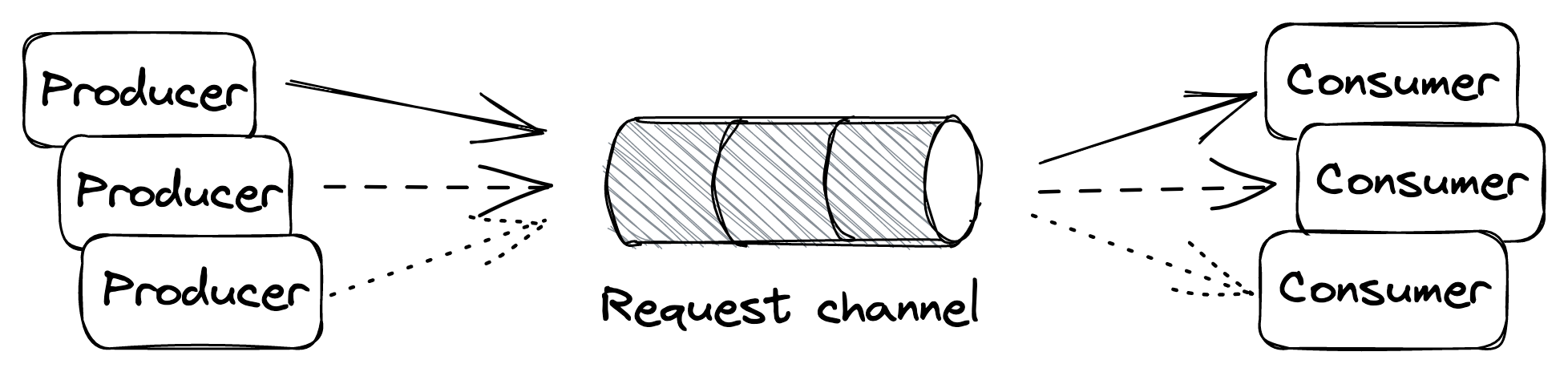
Figure 23.2: One-way messaging style
Request-response messaging
This messaging style is similar to the direct request-response style we are familiar with, albeit with the difference that the request and response messages flow through channels. The consumer has a point-to-point request channel from which it reads messages, while every producer has its dedicated response channel (see Figure 23.3).
When a producer writes a message to the request channel, it decorates it with a request ID and a reference to its response channel. Then, after a consumer has read and processed the message, it writes a reply to the producer’s response channel, tagging it with the request’s ID, which allows the producer to identify the request it belongs to.
Broadcast messaging
In this messaging style, the producer writes a message to a publishsubscribe channel to broadcast it to all consumer instances (see Figure 23.4). This style is generally used to notify a group of processes that a specific event has occurred. For example, we have already encountered this pattern when discussing the outbox pattern in Outbox pattern in Asynchronous transactions.
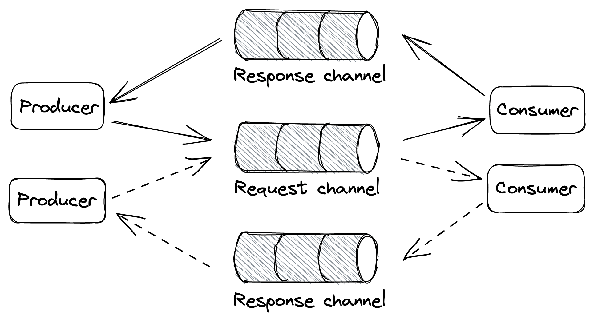
Figure 23.3: Request-response messaging style
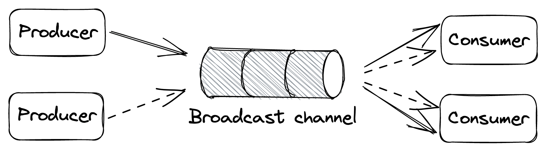
Figure 23.4: Broadcast messaging style
Guarantees
A message channel is implemented by a messaging service, or broker, like AWS SQS[1] or Kafka, which buffers messages and decouples the producer from the consumer. Different message brokers offer different guarantees depending on the tradeoffs their implementations make. For example, you would think that a channel should respect the insertion order of its messages, but you will find that some implementations, like SQS standard queues[2], don’t offer any strong ordering guarantees. Why is that?
Because a message broker needs to scale horizontally just like the applications that use it, its implementation is necessarily distributed. And when multiple nodes are involved, guaranteeing order becomes challenging, as some form of coordination is required. Some brokers, like Kafka, partition a channel into multiple sub-channels. So when messages are written to the channel, they are routed to sub-channels based on their partition key. Since each partition is small enough to be handled by a single broker process, it’s trivial to enforce an ordering of the messages routed to it. But to guarantee that the message order is preserved end-to-end, only a single consumer process is allowed to read from a sub-channel[3].
Because the channel is partitioned, all the caveats discussed in Partitioning (lesson 04.04) apply to it. For example, a partition could become hot enough (due to the volume of incoming messages) that the consumer reading from it can’t keep up with the load. In this case, the channel might have to be rebalanced by adding more partitions, potentially degrading the broker while messages are being shuffled across partitions. It should be clear by now why not guaranteeing the order of messages makes the implementation of a broker much simpler.
Ordering is just one of the many tradeoffs a broker needs to make, such as:
- delivery guarantees, like at-most-once or at-least-once;
- message durability guarantees;
- latency;
- messaging standards supported, like AMQP[4];
- support for competing consumer instances;
- broker limits, such as the maximum supported size of messages.
Because there are so many different ways to implement channels, in the rest of this section, we will make some assumptions for the sake of simplicity:
- Channels are point-to-point and support many producer and consumer instances.
- Messages are delivered to the consumer at least once.
- While a consumer instance is processing a message, the message remains in the channel, but other instances can’t read it for the duration of a visibility timeout. The visibility time-out guarantees that if the consumer instance crashes while processing the message, the message will become visible to other instances when the timeout triggers. When the consumer instance is done processing the message, it deletes it from the channel, preventing it from being received by any other consumer instance in the future.
The above guarantees are similar to the ones offered by managed services such as Amazon’s SQS and Azure Queue Storage[5].
Exactly-once processing
As mentioned before, a consumer instance has to delete a message from the channel once it’s done processing it so that another instance won’t read it. If the consumer instance deletes the message before processing it, there is a risk it could crash after deleting the message but before processing it, causing the message to be lost for good. On the other hand, if the consumer instance deletes the message only after processing it, there is a risk that it crashes after processing the message but before deleting it, causing the same message to be read again later on.
Because of that, there is no such thing[6] as exactly-once message delivery. So the best a consumer can do is to simulate exactly-once message processing by requiring messages to be idempotent and deleting them from the channel only after they have been processed.
Failures
When a consumer instance fails to process a message, the visibility timeout triggers, and the message is eventually delivered to another instance. What happens if processing a specific message consistently fails with an error, though? To guard against the message being picked up repeatedly in perpetuity, we need to limit the maximum number of times the same message can be read from the channel.
To enforce a maximum number of retries, the broker can stamp messages with a counter that keeps track of the number of times the message has been delivered to a consumer. If the broker doesn’t support this functionality out of the box, the consumer can implement it.
Once we have a way to count the number of times a message has been retried, we still have to decide what to do when the maximum is reached. A consumer shouldn’t delete a message without processing it, as that would cause data loss. But what it can do is remove the message from the channel after writing it to a dead letter channel — a channel that buffers messages that have been retried too many times.
This way, messages that consistently fail are not lost forever but merely put on the side so that they don’t pollute the main channel, wasting the consumer’s resources. A human can then inspect these messages to debug the failure, and once the root cause has been identified and fixed, move them back to the main channel to be reprocessed.
Backlogs
One of the main advantages of using a message broker is that it makes the system more robust to outages. This is because the producer can continue writing messages to a channel even if the consumer is temporarily degraded or unavailable. As long as the arrival rate of messages is lower than or equal to their deletion rate, everything is great. However, when that is no longer true and the consumer can’t keep up with the producer, a backlog builds up.
A messaging channel introduces a bimodal behavior in the system. In one mode, there is no backlog, and everything works as expected. In the other, a backlog builds up, and the system enters a degraded state. The issue with a backlog is that the longer it builds up, the more resources and/or time it will take to drain it.
There are several reasons for backlogs, for example:
- more producer instances come online, and/or their throughput increases, and the consumer can’t keep up with the arrival rate;
- the consumer’s performance has degraded and messages take longer to be processed, decreasing the deletion rate;
- the consumer fails to process a fraction of the messages, which are picked up again until they eventually end up in the dead letter channel. This wastes the consumer’s resources and delays the processing of healthy messages.
To detect and monitor backlogs, we can measure the average time a message waits in the channel to be read for the first time. Typically, brokers attach a timestamp of when the message was first written to it. The consumer can use that timestamp to compute how long the message has been waiting in the channel by comparing it to the timestamp taken when the message was read. Although the two timestamps have been generated by two physical clocks that aren’t perfectly synchronized (see Physical clocks in Time), this measure generally provides a good warning sign of backlogs.
Fault isolation
A single producer instance that emits “poisonous” messages that repeatedly fail to be processed can degrade the consumer and potentially create a backlog because these messages are processed multiple times before they end up in the dead-letter channel. Therefore, it’s important to find ways to deal with poisonous messages before that happens.
If messages are decorated with an identifier of the source that generated them, the consumer can treat them differently. For example, suppose messages from a specific user fail consistently. In that case, the consumer could decide to write these messages to an alternate low-priority channel and remove them from the main channel without processing them. The consumer reads from the slow channel but does so less frequently than the main channel, isolating the damage a single bad user can inflict to the others.
Building scalable applications boils down to exploiting three orthogonal patterns:
- breaking the application into separate services, each with its own well-defined responsibility (functional decomposition);
- splitting data into partitions and distributing them across nodes (partitioning);
- replicating functionality or data across nodes (replication).
We have seen plenty of applications of these patterns over the past few chapters. By now, you should have a feel for the pros and cons of each pattern.
There is another message I subtly tried to convey: there is a small subset of managed services that you can use to build a surprisingly large number of applications. The main attraction of managed services is that someone else gets paged for them.[7]
Depending on which cloud provider you are using, the name of the services and their APIs differ somewhat, but conceptually they serve the same use cases. You should be familiar with some way to run your application instances in the cloud (e.g., EC2) and load-balance traffic to them (e.g., ELB). And since you want your applications to be stateless, you also need to be familiar with a file store (e.g., S3), a key-value/document store (e.g., DynamoDB), and a messaging service (e.g., SQS, Kinesis). I would argue that these technologies are reasonable enough defaults for building a large number of scalable applications. Once you have a scalable core, you can add optimizations, such as caching in the form of managed Redis/Memcached or CDNs.
Module references
References
- “Amazon Route 53,” https://aws.amazon.com/route53/
References
- This is an example of the replication pattern in action.
- “HTTP caching,” https://developer.mozilla.org/en-US/docs/Web/HTTP/Caching
- “CQRS,” https://martinfowler.com/bliki/CQRS.html
- This is another instance of functional decomposition.
- “NGINX,” https://www.nginx.com/
- “HAProxy,” https://www.haproxy.com/
References
- “Amazon CloudFront,” https://aws.amazon.com/cloudfront/
- “Akamai,” https://www.akamai.com/
- “The Akamai Network: A Platform for HighPerformance Internet Applications,” https://groups.cs.umass.edu/ramesh/wp-content/uploads/sites/3/2019/12/The-akamai-network-a-platform-for-high-performance-internet-applications.pdf
- “Load Balancing at the Frontend,” https://landing.google.com/sre/sre-book/chapters/load-balancing-frontend/
- “Denial-of-service attack,” https://en.wikipedia.org/wiki/Denial-of-service_attack
- A cache hit occurs when the requested data can be found in the cache, while a cache miss occurs when it cannot.
References
- “Consistent Hashing and Random Trees: Distributed Caching Protocols for Relieving Hot Spots on the World Wide Web,” https://www.cs.princeton.edu/courses/archive/fall09/cos518/papers/chash.pdf
References
- “Amazon Simple Storage Service,” https://aws.amazon.com/s3/
- “Azure Blob Storage,” https://azure.microsoft.com/en-us/services/storage/blobs/#overview
- “Windows Azure Storage: A Highly Available Cloud Storage Service with Strong Consistency,” https://sigops.org/s/conferences/sosp/2011/current/2011-Cascais/printable/11-calder.pdf
- we discussed chain replication in Chain replication in Replication
- “Diving Deep on S3 Consistency,” https://www.allthingsdistributed.com/2021/04/s3-strong-consistency.html
References
- “AWS Well-Architected Framework, Availability,” https://docs.aws.amazon.com/wellarchitected/latest/reliability-pillar/availability.html
- Another way to think about it is that by increasing the number of servers linearly, we increase the availability exponentially.
- “The power of two random choices,” https://brooker.co.za/blog/2012/01/17/two-random.html
- “Autoscaling,” https://docs.microsoft.com/en-us/azure/architecture/best-practices/auto-scaling
- “Implementing health checks,” https://aws.amazon.com/builders-library/implementing-health-checks/
- “Round-robin DNS,” https://en.wikipedia.org/wiki/Round-robin_DNS
- layer 4 is the transport layer in the OSI model
- “SREcon19 Americas - Keeping the Balance: Internet-Scale Loadbalancing Demystified,” https://www.youtube.com/watch?v=woaGu3kJ-xk
- “Network address translation,” https://en.wikipedia.org/wiki/Network_address_translation
- “Introduction to modern network load balancing and proxying,” https://blog.envoyproxy.io/introduction-to-modern-network-load-balancing-and-proxying-a57f6ff80236
- “Anycast,” https://en.wikipedia.org/wiki/Anycast
- “Equal-cost multi-path routing,” https://en.wikipedia.org/wiki/Equal-cost_multi-path_routing
- “Network Load Balancer,” https://aws.amazon.com/elasticloadbalancing/network-load-balancer/
- “Azure Load Balancer,” https://azure.microsoft.com/en-us/services/load-balancer/
- layer 7 is the application layer in the OSI model
- A SYN flood is a form of denial-of-service attack in which an attacker rapidly initiates a TCP connection to a server without finalizing the connection.
- “Service mesh data plane vs. control plane,” https://blog.envoyproxy.io/service-mesh-data-plane-vs-control-plane-2774e720f7fc
- “Service Mesh Wars, Goodbye Istio,” https://blog.polymatic.systems/service-mesh-wars-goodbye-istio-b047d9e533c7
References
- “PostgreSQL Server Configuration, Replication,” https://www.postgresql.org/docs/14/runtime-config-replication.html
- “Amazon RDS Read Replicas,” https://aws.amazon.com/rds/features/read-replicas/
- “Multi-AZ deployments for high availability,” https://docs.aws.amazon.com/AmazonRDS/latest/UserGuide/Concepts.MultiAZ.html
- That said, reducing storage costs isn’t the only benefit of normalization: it also helps maintain data integrity. If a piece of data is duplicated in multiple places, then to update it, we have to make sure it gets updated everywhere. In contrast, if the data is normalized, we only need to update it in one place.
- “Bigtable: A Distributed Storage System for Structured Data,” https://static.googleusercontent.com/media/research.google.com/en//archive/bigtable-osdi06.pdf
- we talked about Dynamo in Dynamo-style data stores in Coordination avoidance
- “AWS re:Invent 2018: Amazon DynamoDB Deep Dive: Advanced Design Patterns for DynamoDB (DAT401),” https://www.youtube.com/watch?v=HaEPXoXVf2k
- On the other hand, while we certainly can find ways to scale a relational database, what works on day 1 might not work on day 10 or 100.
- “Amazon DynamoDB,” https://aws.amazon.com/dynamodb/
- “AWS re:Invent 2018: Amazon DynamoDB Under the Hood: How We Built a Hyper-Scale Database (DAT321),” https://www.youtube.com/watch?v=yvBR71D0nAQ
- “The DynamoDB Book,” https://www.dynamodbbook.com/
- “Andy Pavlo — The official ten-year retrospective of NewSQL databases,” https://www.youtube.com/watch?v=LwkS82zs65g
- “NewSQL database systems are failing to guarantee consistency, and I blame Spanner,” https://dbmsmusings.blogspot.com/2018/09/newsql-database-systems-are-failing-to.html
- “CockroachDB,” https://github.com/cockroachdb/cockroach 15we talked about Spanner in NewSQL in Transactions
References
- “Cache coherence,” https://en.wikipedia.org/wiki/Cache_coherence
- “RocksDB,” http://rocksdb.org/
- “Redis,” https://redis.io/
- “Memcached,” https://memcached.org/
- “Redis cluster tutorial,” https://redis.io/topics/cluster-tutorial
References
- “The Mythical Man-Month,” https://en.wikipedia.org/wiki/The_Mythical_Man-Month
- A more appropriate name for the microservices architecture is service-oriented architecture, but unfortunately, that name comes with some baggage as well.
- This idea is described well in John Ousterhout’s A Philosophy of Software Design, which I highly recommend.
- “MicroservicePremium,” https://martinfowler.com/bliki/MicroservicePremium.html
- “GraphQL,” https://graphql.org/
- “Introduction to JSON Web Tokens,” https://jwt.io/introduction
- “Microservices Security in Action,” https://www.manning.com/books/microservices-security-in-action
- “Azure API Management,” https://azure.microsoft.com/en-gb/services/api-management/
- “Amazon API Gateway,” https://aws.amazon.com/api-gateway/
References
- “Control Planes vs Data Planes,” https://brooker.co.za/blog/2019/03/17/control.html
- “Avoiding overload in distributed systems by putting the smaller service in control,” https://aws.amazon.com/builders-library/avoiding-overload-in-distributed-systems-by-putting-the-smaller-service-in-control/
- This is another example of the CQRS pattern applied in practice.
- That said, there is still the potential to overload the control plane if it needs to juggle too many connections.
- “AWS re:Invent 2018: Close Loops & Opening Minds: How to Take Control of Systems, Big & Small ARC337,” https://www.youtube.com/watch?v=O8xLxNje30M
- That said, having a closed loop doesn’t guarantee that either, it’s merely a pre-requisite.
- “Designing Distributed Control Systems,” https://www.amazon.com/gp/product/1118694155
References
- “Amazon Simple Queue Service,” https://aws.amazon.com/sqs/
- “Amazon SQS Standard queues,” https://docs.aws.amazon.com/AWSSimpleQueueService/latest/SQSDeveloperGuide/standard-queues.html
- This is also referred to as the competing consumer pattern, which is implemented using leader election.
- “Advanced Message Queuing Protocol,” https://en.wikipedia.org/wiki/Advanced_Message_Queuing_Protocol
- “Azure Queue Storage,” https://azure.microsoft.com/en-us/services/storage/queues/
- “You Cannot Have Exactly-Once Delivery Redux,” https://bravenewgeek.com/you-cannot-have-exactly-once-delivery-redux/
- As we will discuss in Maintainability (module 6), maintaining a service is no small feat.