Study one concept at a time. Open the guided module →
Resiliency
Overview: Resiliency
Video coming soon. Start with the reading below.
“Anything that can go wrong will go wrong.”
– Murphy’s law
In the last part, we discussed the three fundamental scalability patterns: functional decomposition, data partitioning, and replication. They all have one thing in common: they increase the number of moving parts (machines, services, processes, etc.) in our applications. But since every part has a probability of failing, the more moving parts there are, the higher the chance that any of them will fail. Eventually, anything that can go wrong will go wrong [8]; power outages, hardware faults, software crashes, memory leaks — you name it.
Remember when we talked about availability and “nines” in Introduction (lesson 01.01)? Well, to guarantee just two nines, an application can only be unavailable for up to 15 minutes a day. That’s very little time to take any manual action when something goes wrong. And if we strive for three nines, we only have 43 minutes per month available. Clearly, the more nines we want, the faster our systems need to detect, react to, and repair faults as they occur. In this part, we will discuss a variety of resiliency best practices and patterns to achieve that.
To build fault-tolerant applications, we first need to have an idea of what can go wrong. In Common failure causes (lesson 05.02), we will explore some of the most common root causes of failures.
Redundancy (lesson 05.03) describes how to use redundancy, the replication of functionality or state, to increase the availability of a system. As we will learn, redundancy is only helpful when the redundant nodes can’t fail for the same reason at the same time, i.e., when failures are not correlated.
Fault isolation (lesson 05.04) discusses how to isolate correlated failures by partitioning resources and then describes two very powerful forms of partitioning: shuffle sharding and cellular architectures.
Downstream resiliency (lesson 05.05) dives into more tactical resiliency patterns for tolerating failures of downstream dependencies that you can apply to existing systems with few changes, like timeouts and retries.
Upstream resiliency (lesson 05.06) discusses resiliency patterns, like load shedding and rate-limiting, for protecting systems against overload from upstream dependencies.
Common failure causes
Video coming soon. Start with the reading below.
We say that a system has a failure[1] when it no longer provides a service to its users that meets its specification. A failure is caused by a fault: a failure of an internal component or an external dependency the system depends on. Some faults can be tolerated and have no user-visible impact at all, while others lead to failures.
To build fault-tolerant applications, we first need to have an idea of what can go wrong. In the next few sections, we will explore some of the most common root causes of failures. By the end of it, you will likely wonder how to tolerate all these different types of faults. The answers will follow in the next few chapters.
Hardware faults
Any physical part of a machine can fail. HDDs, memory modules, power supplies, motherboards, SSDs, NICs, or CPUs, can all stop working for various reasons. In some cases, hardware faults can cause data corruption as well. If that wasn’t enough, entire data centers can go down because of power cuts or natural disasters.
As we will discuss later, we can address many of these infrastructure faults with redundancy. You would think that these faults are the main cause for distributed applications failing, but in reality, they often fail for very mundane reasons.
Incorrect error handling
A study from 2014[2] of user-reported failures from five popular distributed data stores found that the majority of catastrophic failures were the result of incorrect handling of non-fatal errors.
In most cases, the bugs in the error handling could have been detected with simple tests. For example, some handlers completely ignored errors. Others caught an overly generic exception, like Exception in Java, and aborted the entire process for no good reason. And some other handlers were only partially implemented and even contained “FIXME” and “TODO” comments.
In hindsight, this is perhaps not too surprising, given that error handling tends to be an afterthought.[3] Later, in Testing (lesson 06.02), we will take a closer look at best practices for testing large distributed applications.
Configuration changes
Configuration changes are one of the leading root causes for catastrophic failures[4]. It’s not just misconfigurations that cause problems, but also valid configuration changes to enable rarely-used features that no longer work as expected (or never did).
What makes configuration changes particularly dangerous is that their effects can be delayed[5]. If an application reads a configuration value only when it’s actually needed, an invalid value might take effect only hours or days after it has changed and thus escape early detection.
This is why configuration changes should be version-controlled, tested, and released just like code changes, and their validation should happen preventively when the change happens. In Continuous delivery and deployment (lesson 06.03), we will discuss safe release practices for code and configuration changes in the context of continuous deployments.
Single points of failure
A single point of failure (SPOF) is a component whose failure brings the entire system down with it. In practice, systems can have multiple SPOFs.
Humans make for great SPOFs, and if you put them in a position where they can cause a catastrophic failure on their own, you can bet they eventually will. For example, human failures often happen when someone needs to manually execute a series of operational steps in a specific order without making any mistakes. On the other hand, computers are great at executing instructions, which is why automation should be leveraged whenever possible.
Another common SPOF is DNS[6]. If clients can’t resolve the domain name for an application, they won’t be able to connect to it. There are many reasons why that can happen, ranging from domain names expiring[7] to entire root level domains going down[8].
Similarly, the TLS certificate used by an application for its HTTP endpoints is also a SPOF[9]. If the certificate expires, clients won’t be able to open a secure connection with the application.
Ideally, SPOFs should be identified when the system is designed. The best way to detect them is to examine every system component and ask what would happen if it were to fail. Some SPOFs can be architected away, e.g., by introducing redundancy, while others can’t. In that case, the only option left is to reduce the SPOF’s blast radius, i.e., the damage the SPOF inflicts on the system when it fails. Many of the resiliency patterns we will discuss later reduce the blast radius of failures.
Network faults
When a client sends a request to a server, it expects to receive a response from it a while later. In the best case, it receives the response shortly after sending the request. If that doesn’t happen, the client has two options: continue to wait or fail the request with a time-out exception or error.
As discussed in Failure detection (lesson 03.03), when the concepts of failure detection and timeouts were introduced, there are many reasons for not getting a prompt response. For example, the server could be very slow or have crashed while processing the request; or maybe the network could be losing a small percentage of packets, causing lots of retransmissions and delays.
Slow network calls are the silent killers[10] of distributed systems. Because the client doesn’t know whether the response will eventually arrive, it can spend a long time waiting before giving up, if it gives up at all, causing performance degradations that are challenging to debug. This kind of fault is also referred to as a gray failure[11]: a failure that is so subtle that it can’t be detected quickly or accurately. Because of their nature, gray failures can easily bring an entire system down to its knees.
In the next section, we will explore another common cause of gray failures.
Resource leaks
From an observer’s point of view, a very slow process is not very different from one that isn’t running at all — neither can perform useful work. Resource leaks are one of the most common causes of slow processes.
Memory is arguably the most well-known resource affected by leaks. A memory leak causes a steady increase in memory consumption over time. Even languages with garbage collection are vulnerable to leaks: if a reference to an object that is no longer needed is kept somewhere, the garbage collector won’t be able to delete it. When a leak has consumed so much memory that there is very little left, the operating system will start to swap memory pages to disk aggressively. Also, the garbage collector will kick in more frequently, trying to release memory. All of this consumes CPU cycles and makes the process slower. Eventually, when there is no more physical memory left, and there is no more space in the swap file, the process won’t be able to allocate memory, and most operations will fail.
Memory is just one of the many resources that can leak. Take thread pools, for example: if a thread acquired from a pool makes a synchronous blocking HTTP call without a timeout and the call never returns, the thread won’t be returned to the pool. And since the pool has a limited maximum size, it will eventually run out of threads if it keeps losing them.
You might think that making asynchronous calls rather than synchronous ones would help in the previous case. However, modern HTTP clients use socket pools to avoid recreating TCP connections and paying a performance fee, as discussed in Reliable links (lesson 02.02). If a request is made without a timeout, the connection is never returned to the pool. As the pool has a limited maximum size, eventually, there won’t be any connections left.
On top of that, your code isn’t the only thing accessing memory, threads, and sockets. The libraries your application depends on use the same resources, and they can hit the same issues we just discussed.
Load pressure
Every system has a limit of how much load it can withstand, i.e., its capacity. So when the load directed to the system continues to increase, it’s bound to hit that limit sooner or later. But an organic increase in load, that gives the system the time to scale out accordingly and increase its capacity, is one thing, and a sudden and unexpected flood is another.
For example, consider the number of requests received by an application in a period of time. The rate and the type of incoming requests can change over time, and sometimes suddenly, for a variety of reasons:
- The requests might have a seasonality. So, for example, depending on the hour of the day, the application is hit by users in different countries.
- Some requests are much more expensive than others and abuse the system in unexpected ways, like scrapers slurping in data at super-human speed.
- Some requests are malicious, like those of DDoS attacks that try to saturate the application’s bandwidth to deny legitimate users access to it.
While some load surges can be handled by automation that adds capacity (e.g., autoscaling), others require the system to reject requests to shield it from overloading, using the patterns we will discuss in Upstream resiliency (lesson 05.06).
Cascading failures
You would think that if a system has hundreds of processes, it shouldn’t make much of a difference if a small percentage are slow or unreachable. The thing about faults is that they have the potential to spread virally and cascade from one process to the other until the whole system crumbles to its knees. This happens when system components depend on each other, and a failure in one increases the probability of failure in others.
For example, suppose multiple clients are querying two database replicas, A and B, behind a load balancer. Each replica handles about 50 transactions per second (see Figure 24.1).
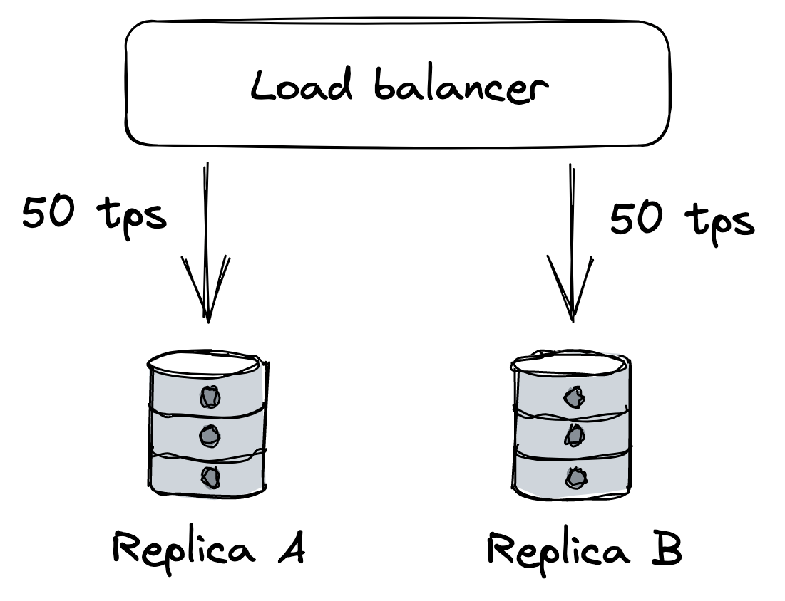
Figure 24.1: Two replicas behind a load balancer; each is handling half the load.
Suddenly, replica B becomes unavailable because of a network fault. The load balancer detects that B is unavailable and removes it from the pool. Because of that, replica A has to pick up the slack for B and serve twice the requests per unit time it was serving before (see Figure 24.2).
If replica A struggles to keep up with the incoming requests, the clients will experience increasingly more timeouts and start to retry requests, adding more load to the system. Eventually, replica A will be under so much load that most requests will time out, forcing the load balancer to remove it from the pool. In other words, the original network fault that caused replica B to become unavailable cascaded into a fault at replica A.
Suppose now that replica B becomes available again and the load balancer puts it back in the pool. Because it’s the only replica in the pool, it will be flooded with requests, causing it to overload and eventually be removed again.
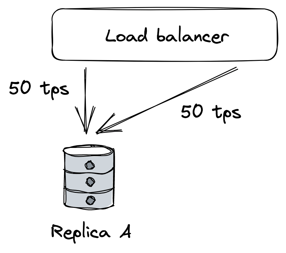
Figure 24.2: When replica B becomes unavailable, A will be hit with more load, which can strain it beyond its capacity.
You can see how even after the network fault is gone, the application continues to struggle because of a feedback loop that causes the load to jump from one replica to another. Failures with this characteristic are also referred to as metastable[12].
A big enough corrective action is usually needed to break the loop, like temporarily blocking traffic from getting to the replicas in the first place. Unfortunately, these failures are very hard to mitigate once they have started, and the best way to prevent them is to stop faults from spreading from one component to another in the first place.
Managing risk
As it should be evident by now, a distributed application needs to accept that faults are inevitable and be prepared to detect, react to, and repair them as they occur.
At this point, you might feel overwhelmed by the sheer amount of things that can go wrong. But just because a specific fault has a chance of happening, it doesn’t mean we have to do something about it. We first have to consider the probability it will manifest and the impact it will cause to the system’s users when it does. By multiplying the two factors together, we get a risk score[13] that we can use to prioritize which faults to address (see Figure 24.3) first. For example, a fault that is very likely to happen, and has a large impact, should be tackled head on; on the other hand, a fault with a low likelihood and low impact can wait.
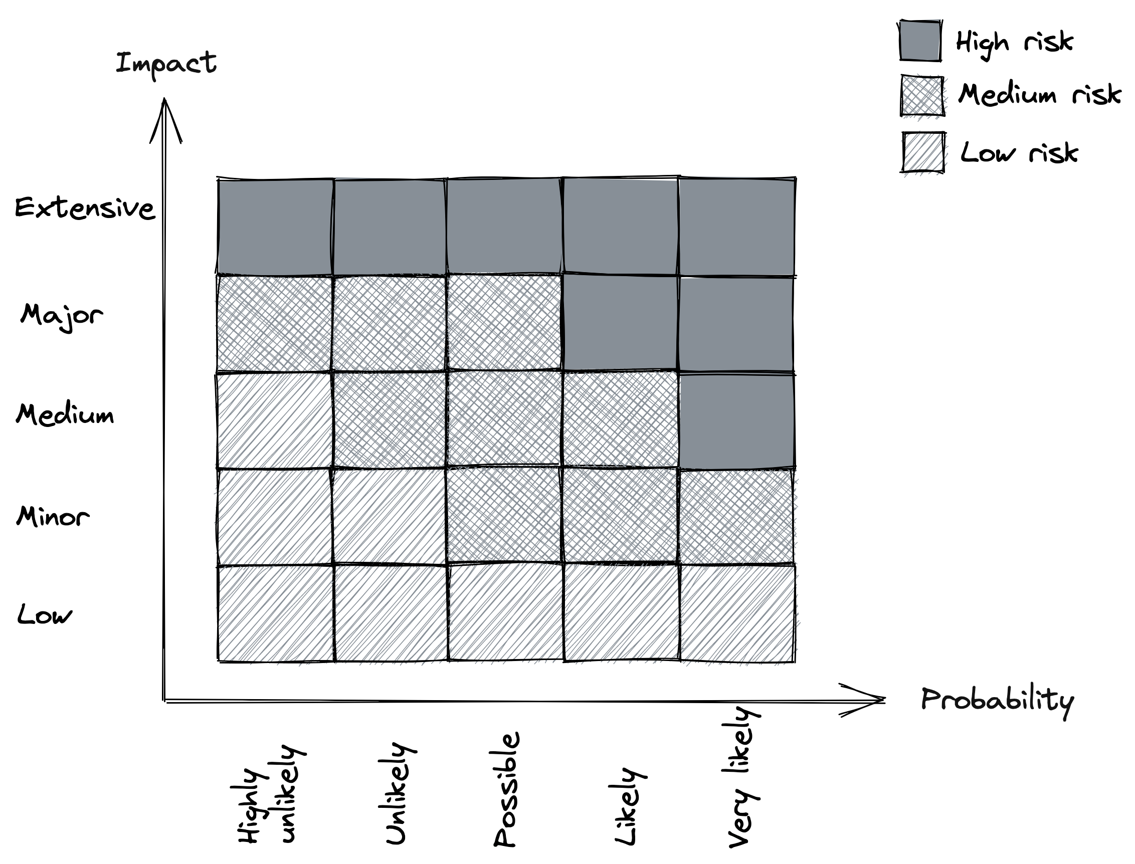
Figure 24.3: Risk matrix
Once we decide that we need to do something about a specific fault, we can try to reduce its probability and/or reduce its impact. This will be the main focus of the following lessons.
Redundancy
Video coming soon. Start with the reading below.
Redundancy, the replication of functionality or state, is arguably the first line of defense against failures. When functionality or state is replicated over multiple nodes and a node fails, the others can take over. Moreover, as discussed in Scalability (module 4), replication is also a core pattern that enables our applications to scale out horizontally.
Redundancy is the main reason why distributed applications can achieve better availability than single-node applications. But only some forms of redundancy actually improve availability. Marc Brooker lists four prerequisites[1]:
- The complexity added by introducing redundancy mustn’t cost more availability than it adds.
- The system must reliably detect which of the redundant components are healthy and which are unhealthy.
- The system must be able to run in degraded mode.
- The system must be able to return to fully redundant mode.
Let’s see how these prerequisites apply to a concrete example. Hardware faults such as disk, memory, and network failures can cause a node to crash, degrade or become otherwise unavailable. In a stateless service, a load balancer can mask these faults using a pool of redundant nodes. Although the load balancer increases the system’s complexity and, therefore, the number of ways the system can fail, the benefits in terms of scalability and availability almost always outweigh the risks it introduces (e.g., the load balancer failing).
The load balancer needs to detect which nodes are healthy and which aren’t to take the faulty ones out of the pool. It does that with health checks, as we learned in Network load balancing (lesson 04.06). Health checks are critical to achieving high availability; if there are ten servers in the pool and one is unresponsive for some reason, then 10% of requests will fail, causing the availability to drop. Therefore, the longer it takes for the load balancer to detect the unresponsive server, the longer the failures will be visible to the clients.
Now, when the load balancer takes one or more unhealthy servers out of the pool, the assumption is that the others have enough capacity left to handle the increase in load. In other words, the system must be able to run in degraded mode. However, that by itself is not enough; new servers also need to be added to the pool to replace the ones that have been removed. Otherwise, there eventually won’t be enough servers left to cope with the load.
In stateful services, masking a node failure is a lot more complex since it involves replicating state. We have discussed replication at length in the earlier lessons, and it shouldn’t come as a surprise by now that meeting the above requisites is a lot more challenging for a stateful service than for a stateless one.
Correlation
Redundancy is only helpful when the redundant nodes can’t fail for the same reason at the same time, i.e., when failures are not correlated. For example, if a faulty memory module causes a server to crash, it’s unlikely other servers will fail simultaneously for the same reason since they are running on different machines. However, if the servers are hosted in the same data center, and a fiber cut or an electrical storm causes a data-center-wide outage, the entire application becomes unavailable no matter how many servers there are. In other words, the failures caused by a data center outage are correlated and limit the application’s availability. So if we want to increase the availability, we have to reduce the correlation between failures by using more than one data center.
Cloud providers such as AWS and Azure replicate their entire stack in multiple regions for that very reason. Each region comprises multiple data centers called Availability Zones (AZs) that are cross-connected with high-speed network links. AZs are far enough from each other to minimize the risk of correlated failures (e.g., power cuts) but still close enough to have low network latency, which is bounded by the speed of light. In fact, the latency is low enough by design to support synchronous replication protocols without a significant latency penalty.
With AZs, we can create applications that are resilient to data center outages. For example, a stateless service could have instances running in multiple AZs behind a shared load balancer so that if an AZ becomes unavailable, it doesn’t impact the availability of the service. On the other hand, stateful services require the use of a replication protocol to keep their state in sync across AZs. But since latencies are low enough between AZs, the replication protocol can be partially synchronous, like Raft, or even fully synchronous, like chain replication.
Taking it to the extreme, a catastrophic event could destroy an entire region with all of its AZs. To tolerate that, we can duplicate the entire application stack in multiple regions. To distribute the traffic to different data centers located in different regions, we can use global DNS load balancing. Unlike earlier, the application’s state needs to be replicated asynchronously across regions[2] given the high network latency between regions (see Figure 25.1).
That said, the chance of an entire region being destroyed is extremely low. Before embarking on the effort of making your application resilient against region failures, you should have very good
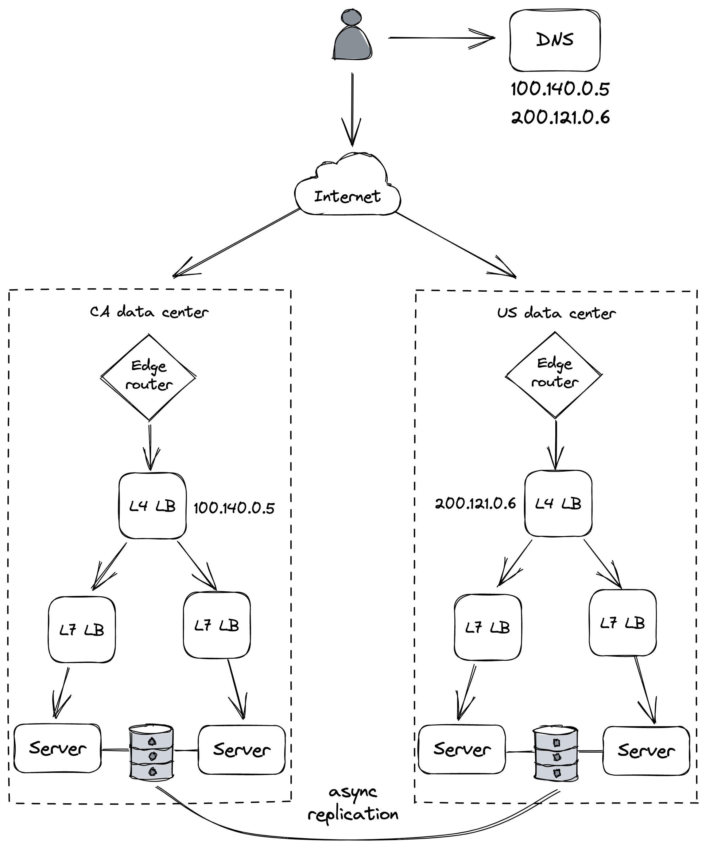
Figure 25.1: A simplistic multi-region architecture
reasons for it. It’s more likely your application will be forced to have a presence in multiple regions for legal compliance reasons. For example, there are laws mandating that the data of European customers has to be processed and stored within Europe[3].
Fault isolation
Video coming soon. Start with the reading below.
So far, we have discussed how to address infrastructure faults with redundancy, but there are other kinds of failures that we can’t tolerate with redundancy alone because of their high degree of correlation.
For example, suppose a specific user sends malformed requests (deliberately or not) that cause the servers handling them to crash because of a bug. Since the bug is in the code, it doesn’t matter how many DCs and regions our application is deployed to; if the user’s requests can land anywhere, they can affect all DCs and regions. Due to their nature, these requests are sometimes referred to as poison pills.
Similarly, if the requests of a specific user require a lot more resources than others, they can degrade the performance for every other user (aka noisy neighbor effect).
The main issue in the previous examples is that the blast radius of poison pills and noisy neighbors is the entire application. To reduce it, we can partition the application’s stack by user so that the requests of a specific user can only ever affect the partition it was assigned to.[1] That way, even if a user is degrading a partition, the issue is isolated from the rest of the system.
For example, suppose we have 6 instances of a stateless service behind a load balancer, divided into 3 partitions (see Figure 26.1). In this case, a noisy or poisonous user can only ever impact 33 percent of users. And as the number of partitions increases, the blast radius decreases further.
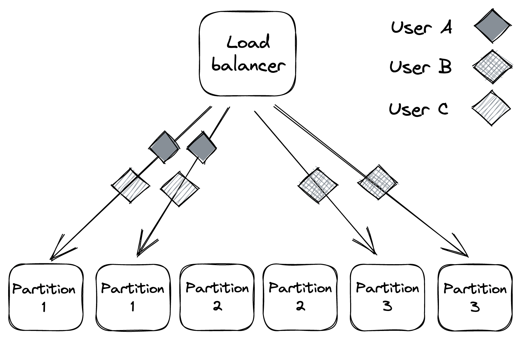
Figure 26.1: Service instances partitioned into 3 partitions
The use of partitions for fault isolation is also referred to as the bulkhead pattern, named after the compartments of a ship’s hull. If one compartment is damaged and fills up with water, the leak is isolated to that partition and doesn’t spread to the rest of the ship.
Shuffle sharding
The problem with partitioning is that users who are unlucky enough to land on a degraded partition are impacted as well. For stateless services, there is a very simple, yet powerful, variation of partitioning called shuffle sharding[2] that can help mitigate that.
The idea is to introduce virtual partitions composed of random (but permanent) subsets of service instances. This makes it much more unlikely for two users to be allocated to the same partition as each other.
Let’s go back to our previous example of a stateless service with 6 instances. How many combinations of virtual partitions with 2 instances can we build out of 6 instances? If you recall the combinations formula from your high school statistics class, the answer is 15:
n! r!(n−r)! = 6!
2!4! = 15
There are now 15 partitions for a user to be assigned to, while before, we had only 3, which makes it a lot less likely for two users to end up in the same partition. The caveat is that virtual partitions partially overlap (see Figure 26.2). But by combining shuffle sharding with a load balancer that removes faulty instances, and clients that retry failed requests, we can build a system with much better fault isolation than one with physical partitions alone.
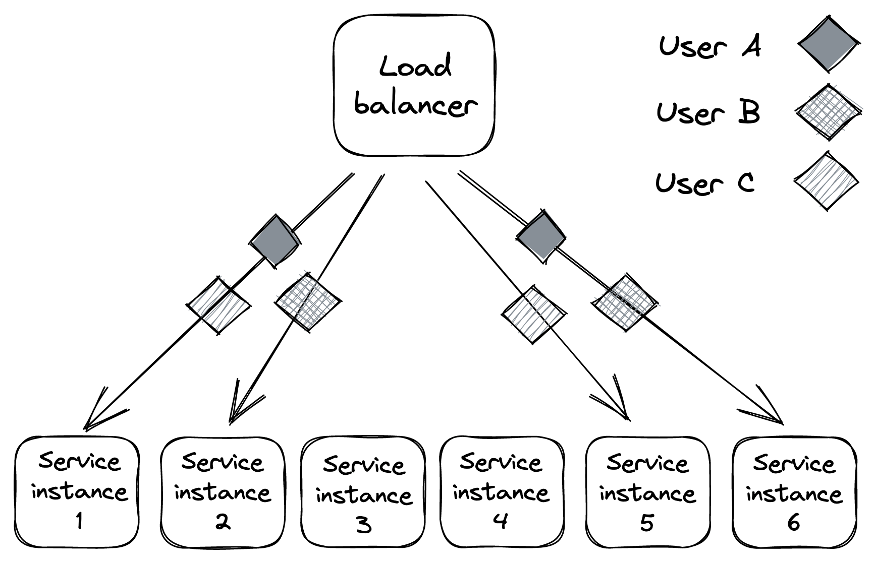
Figure 26.2: Virtual partitions are far less likely to fully overlap with each other.
Cellular architecture
In the previous examples, we discussed partitioning in the context of stateless services. We can take it up a notch and partition the entire application stack, including its dependencies (load balancers, compute services, storage services, etc.), by user[3] into cells[4]. Each cell is completely independent of others, and a gateway service is responsible for routing requests to the right cells.
We have already seen an example of a “cellular” architecture when discussing Azure Storage in File storage (lesson 04.05). In Azure Storage, a cell is a storage cluster, and accounts are partitioned across storage clusters (see Figure 26.3).
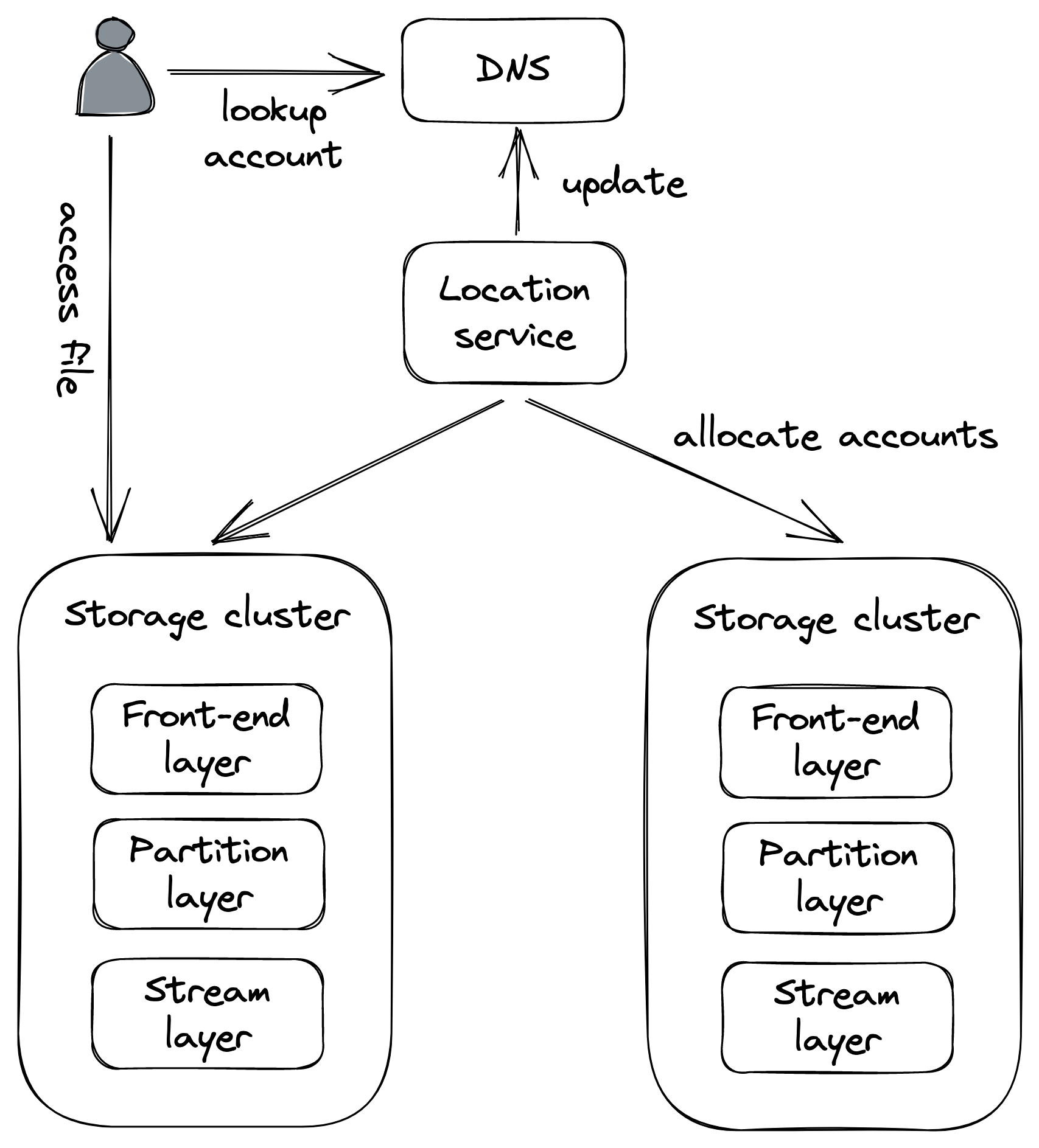
Figure 26.3: Each storage cluster (stamp) is a cell in Azure Storage.
An unexpected benefit of cellular architectures comes from setting limits to the maximum capacity of a cell. That way, when the system needs to scale out, a new cell is added rather than scaling out existing ones. Since a cell has a maximum size, we can thoroughly test and benchmark it at that size, knowing that we won’t have any surprises in the future and hit some unexpected brick wall.
Downstream resiliency
Video coming soon. Start with the reading below.
Now that we have discussed how to reduce the impact of faults at the architectural level with redundancy and partitioning, we will dive into tactical resiliency patterns that stop faults from propagating from one component or service to another. In this lesson, we will discuss patterns that protect a service from failures of downstream dependencies.
Timeout
When a network call is made, it’s best practice to configure a time-out to fail the call if no response is received within a certain amount of time. If the call is made without a timeout, there is a chance it will never return, and as mentioned in Common failure causes (lesson 05.02), network calls that don’t return lead to resource leaks. Thus, the role of timeouts is to detect connectivity faults and stop them from cascading from one component to another. In general, timeouts are a must-have for operations that can potentially never return, like acquiring a mutex.
Unfortunately, some network APIs don’t have a way to set a time-out in the first place, while others have no timeout configured by default. For example, JavaScript’s XMLHttpRequest is the web API to retrieve data from a server asynchronously, and its default time-out is zero[1], which means there is no timeout:
var xhr = new XMLHttpRequest();
xhr.open("GET", "/api", true);
// No timeout by default, so it needs to be set explicitly!
xhr.timeout = 10000; // 10K milliseconds
xhr.onload = function () {
  // Request finished
};
xhr.ontimeout = function (e) {
  // Request timed out
};
xhr.send(null);
The fetch web API is a modern replacement for XMLHttpRequest that uses Promises. When the fetch API was initially introduced, there was no way to set a timeout at all[2]. Browsers have only later added support for timeouts through the Abort API[3]. Things aren’t much rosier for Python; the popular requests library uses a default timeout of infinity[4]. And Go’s HTTP package doesn’t use timeouts[5] by default.
Modern HTTP clients for Java and .NET do a better job and usually, come with default timeouts. For example, .NET Core HttpClient has a default timeout of 100 seconds[6]. It’s lax but arguably better than not having a timeout at all.
As a rule of thumb, always set timeouts when making network calls, and be wary of third-party libraries that make network calls but don’t expose settings for timeouts.
But how do we determine a good timeout duration? One way is to base it on the desired false timeout rate[7]. For example, suppose we have a service calling another, and we are willing to accept that 0.1% of downstream requests that would have eventually returned a response time out (i.e., 0.1% false timeout rate). To accomplish that, we can configure the timeout based on the 99.9th percentile of the downstream service’s response time.
We also want to have good monitoring in place to measure the entire lifecycle of a network call, like the duration of the call, the status code received, and whether a timeout was triggered. We will talk more about monitoring later in this learning path, but the point I want to make here is that we have to measure what happens at the integration points of our systems, or we are going to have a hard time debugging production issues.
Ideally, a network call should be wrapped within a library function that sets a timeout and monitors the request so that we don’t have to remember to do this for each call. Alternatively, we can also use a reverse proxy co-located on the same machine, which intercepts remote calls made by our process. The proxy can enforce timeouts and monitor calls, relieving our process ofthis responsibility. We talked about this in Application layer load balancing in Network load balancing when discussing the sidecar pattern and the service mesh.
Retry
We know by now that a client should configure a timeout when making a network request. But what should it do when the request fails or times out? The client has two options at that point: it can either fail fast or retry the request. If a short-lived connectivity issue caused the failure or timeout, then retrying after some backoff time has a high probability of succeeding. However, if the downstream service is overwhelmed, retrying immediately after will only worsen matters. This is why retrying needs to be slowed down with increasingly longer delays between the individual retries until either a maximum number of retries is reached or enough time has passed since the initial request.
Exponential backoff
To set the delay between retries, we can use a capped exponential function, where the delay is derived by multiplying the initial backoff duration by a constant that increases exponentially after each attempt, up to some maximum value (the cap):
delay = min(cap, initial-backoff ⋅2attempt)
For example, if the cap is set to 8 seconds, and the initial backoff duration is 2 seconds, then the first retry delay is 2 seconds, the second is 4 seconds, the third is 8 seconds, and any further delay will be capped to 8 seconds.
Although exponential backoff does reduce the pressure on the downstream dependency, it still has a problem. When the downstream service is temporarily degraded, multiple clients will likely see their requests failing around the same time. This will cause clients to retry simultaneously, hitting the downstream service with load spikes that further degrade it, as shown in Figure 27.1.
To avoid this herding behavior, we can introduce random jitter[8] into the delay calculation. This spreads retries out over time, smoothing out the load to the downstream service:
delay = random(0, min(cap, initial-backoff ⋅2attempt))
Actively waiting and retrying failed network requests isn’t the only way to implement retries. In batch applications that don’t have strict real-time requirements, a process can park a failed
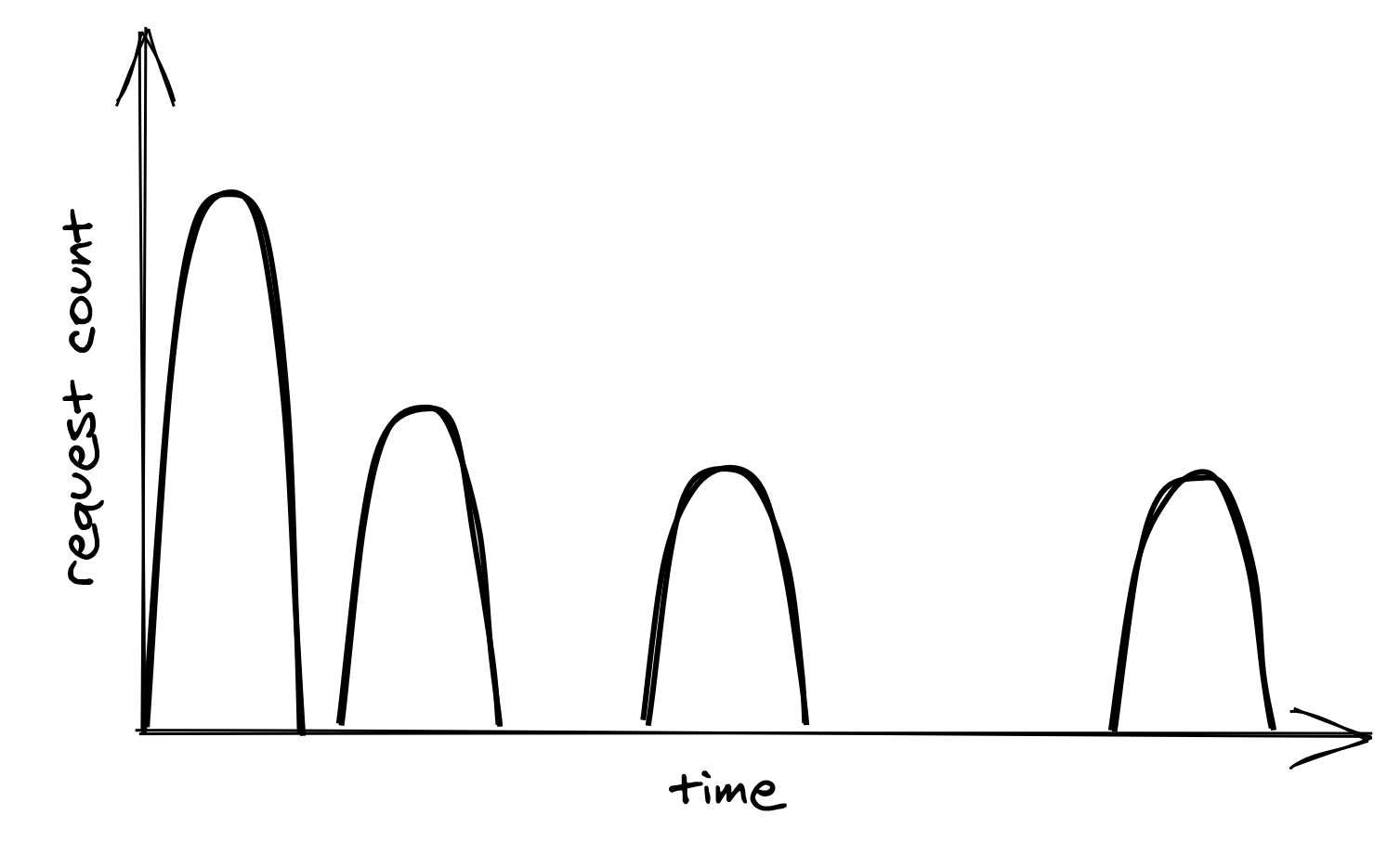
Figure 27.1: Retry storm
request into a retry queue. The same process, or possibly another, can read from the same queue later and retry the failed requests.
Just because a network call can be retried doesn’t mean it should be. If the error is not short-lived, for example, because the process is not authorized to access the remote endpoint, it makes no sense to retry the request since it will fail again. In this case, the process should fail fast and cancel the call right away. And as discussed in Idempotency in APIs, we should also understand the consequences of retrying a network call that isn’t idempotent and whose side effects can affect the application’s correctness.
Retry amplification
Suppose that handling a user request requires going through a chain of three services. The user’s client calls service A, which calls service B, which in turn calls service C. If the intermediate request from service B to service C fails, should B retry the request or not? Well, if B does retry it, A will perceive a longer execution time for its request, making it more likely to hit A’s timeout. If that happens, A retries the request, making it more likely for the client to hit its timeout and retry.
Having retries at multiple levels of the dependency chain can amplify the total number of retries — the deeper a service is in the chain, the higher the load it will be exposed to due to retry amplification (see Figure 27.2).
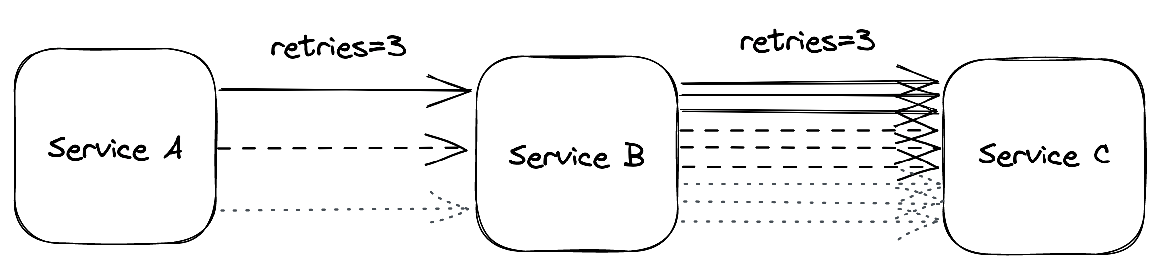
Figure 27.2: Retry amplification in action
And if the pressure gets bad enough, this behavior can easily overload downstream services. That’s why, when we have long dependency chains, we should consider retrying at a single level of the chain and failing fast in all the others.
Circuit breaker
Suppose a service uses timeouts to detect whether a downstream dependency is unavailable and retries to mitigate transient failures. If the failures aren’t transient and the downstream dependency remains unresponsive, what should it do then? If the service keeps retrying failed requests, it will necessarily become slower for its clients. In turn, this slowness can spread to the rest of the system.
To deal with non-transient failures, we need a mechanism that detects long-term degradations of downstream dependencies and stops new requests from being sent downstream in the first place. After all, the fastest network call is the one we don’t have to make. The mechanism in question is the circuit breaker, inspired by the same functionality implemented in electrical circuits.
The goal of the circuit breaker is to allow a sub-system to fail without slowing down the caller. To protect the system, calls to the failing sub-system are temporarily blocked. Later, when the subsystem recovers and failures stop, the circuit breaker allows calls to go through again.
Unlike retries, circuit breakers prevent network calls entirely, making the pattern particularly useful for non-transient faults. In other words, retries are helpful when the expectation is that the next call will succeed, while circuit breakers are helpful when the expectation is that the next call will fail.
A circuit breaker can be implemented as a state machine with three states: open, closed, and half-open (see Figure 27.3).
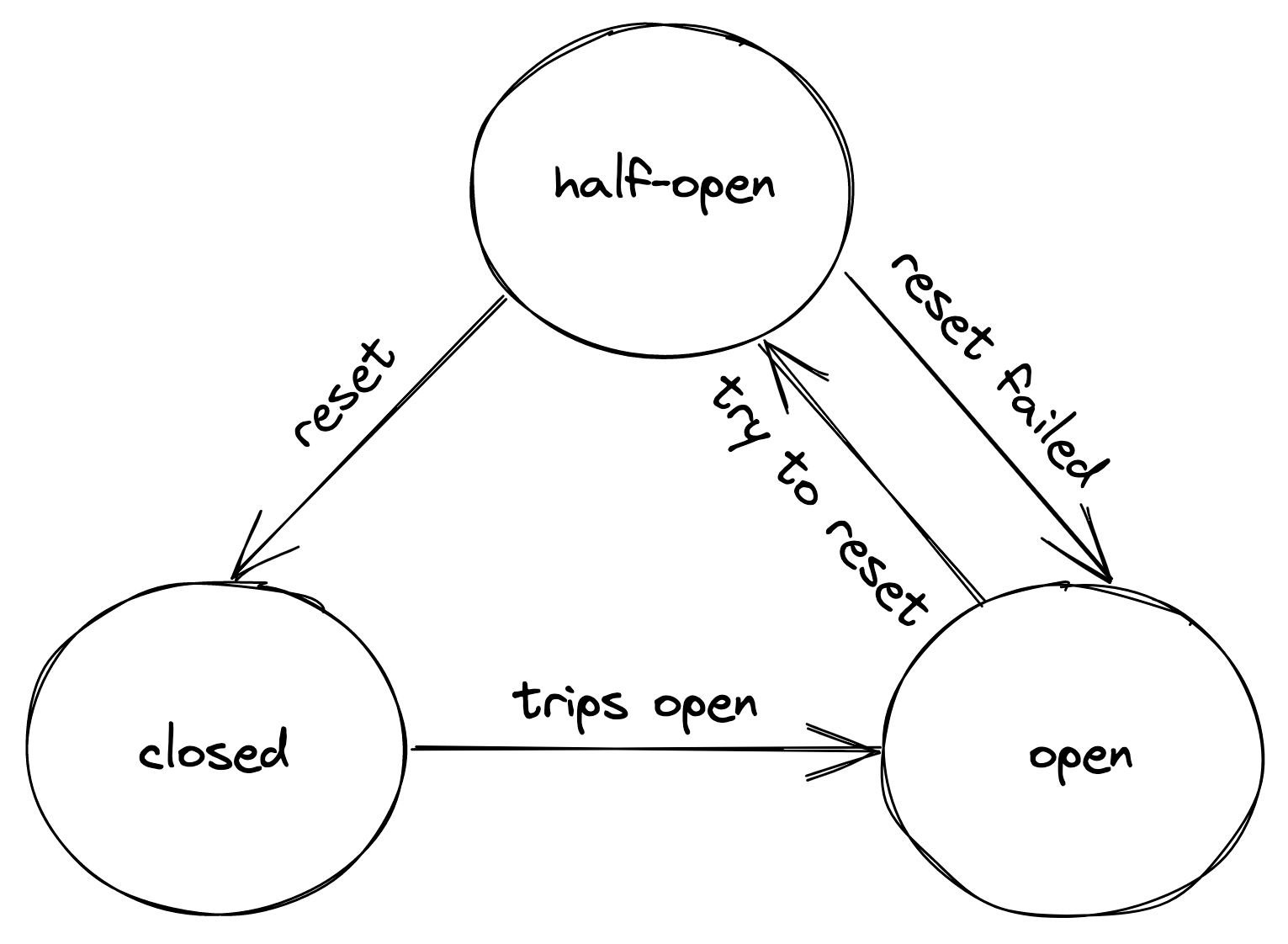
Figure 27.3: Circuit breaker state machine
In the closed state, the circuit breaker merely acts as a pass-through for network calls. In this state, the circuit breaker tracks the number of failures, like errors and timeouts. If the number goes over a certain threshold within a predefined time interval, the circuit breaker trips and opens the circuit.
When the circuit is open, network calls aren’t attempted and fail immediately. As an open circuit breaker can have business implications, we need to consider what should happen when a downstream dependency is down. If the dependency is non-critical, we want our service to degrade gracefully rather than to stop entirely. Think of an airplane that loses one of its non-critical sub-systems in flight; it shouldn’t crash but rather gracefully degrade to a state where the plane can still fly and land. Another example is Amazon’s front page; if the recommendation service is unavailable, the page renders without recommendations. It’s a better outcome than failing to render the whole page entirely.
After some time has passed, the circuit breaker gives the downstream dependency another chance and transitions to the half-open state. In the half-open state, the next call is allowed to pass through to the downstream service. If the call succeeds, the circuit breaker transitions to the closed state; if the call fails instead, it transitions back to the open state.
You might think that’s all there is to understand how a circuit breaker works, but the devil is in the details. For example, how many failures are enough to consider a downstream dependency down? How long should the circuit breaker wait to transition from the open to the half-open state? It really depends on the specific context; only by using data about past failures can we make an informed decision.
Upstream resiliency
Video coming soon. Start with the reading below.
The previous lesson discussed patterns that protect services against downstream failures, like failures to reach an external dependency. In this lesson, we will shift gears and discuss mechanisms to protect against upstream pressure.[1]
Load shedding
A server has very little control over how many requests it receives at any given time. The operating system has a connection queue per port with a limited capacity that, when reached, causes new connection attempts to be rejected immediately. But typically, under extreme load, the server crawls to a halt before that limit is reached as it runs out of resources like memory, threads, sockets, or files. This causes the response time to increase until eventually, the server becomes unavailable to the outside world.
When a server operates at capacity, it should reject excess requests[2] so that it can dedicate its resources to the requests it’s already processing. For example, the server could use a counter to measure the number of concurrent requests being processed that is incremented when a new request comes in and decreased when a response is sent. The server can then infer whether it’s overloaded by comparing the counter with a threshold that approximates the server’s capacity.
When the server detects that it’s overloaded, it can reject incoming requests by failing fast and returning a response with status code 503 (Service Unavailable). This technique is also referred to as load shedding. The server doesn’t necessarily have to reject arbitrary requests; for example, if different requests have different priorities, the server could reject only low-priority ones. Alternatively, the server could reject the oldest requests first since those will be the first ones to time out and be retried, so handling them might be a waste of time.
Unfortunately, rejecting a request doesn’t completely shield the server from the cost of handling it. Depending on how the rejection is implemented, the server might still have to pay the price of opening a TLS connection and reading the request just to reject it. Hence, load shedding can only help so much, and if load keeps increasing, the cost of rejecting requests will eventually take over and degrade the server.
Load leveling
There is an alternative to load shedding, which can be exploited when clients don’t expect a prompt response. The idea is to introduce a messaging channel between the clients and the service. The channel decouples the load directed to the service from its capacity, allowing it to process requests at its own pace.
This pattern is referred to as load leveling and it’s well suited to fending off short-lived spikes, which the channel smooths out (see Figure 28.1). But if the service doesn’t catch up eventually, a large backlog will build up, which comes with its own problems, as discussed in Messaging (lesson 04.11).
Load-shedding and load leveling don’t address an increase in load
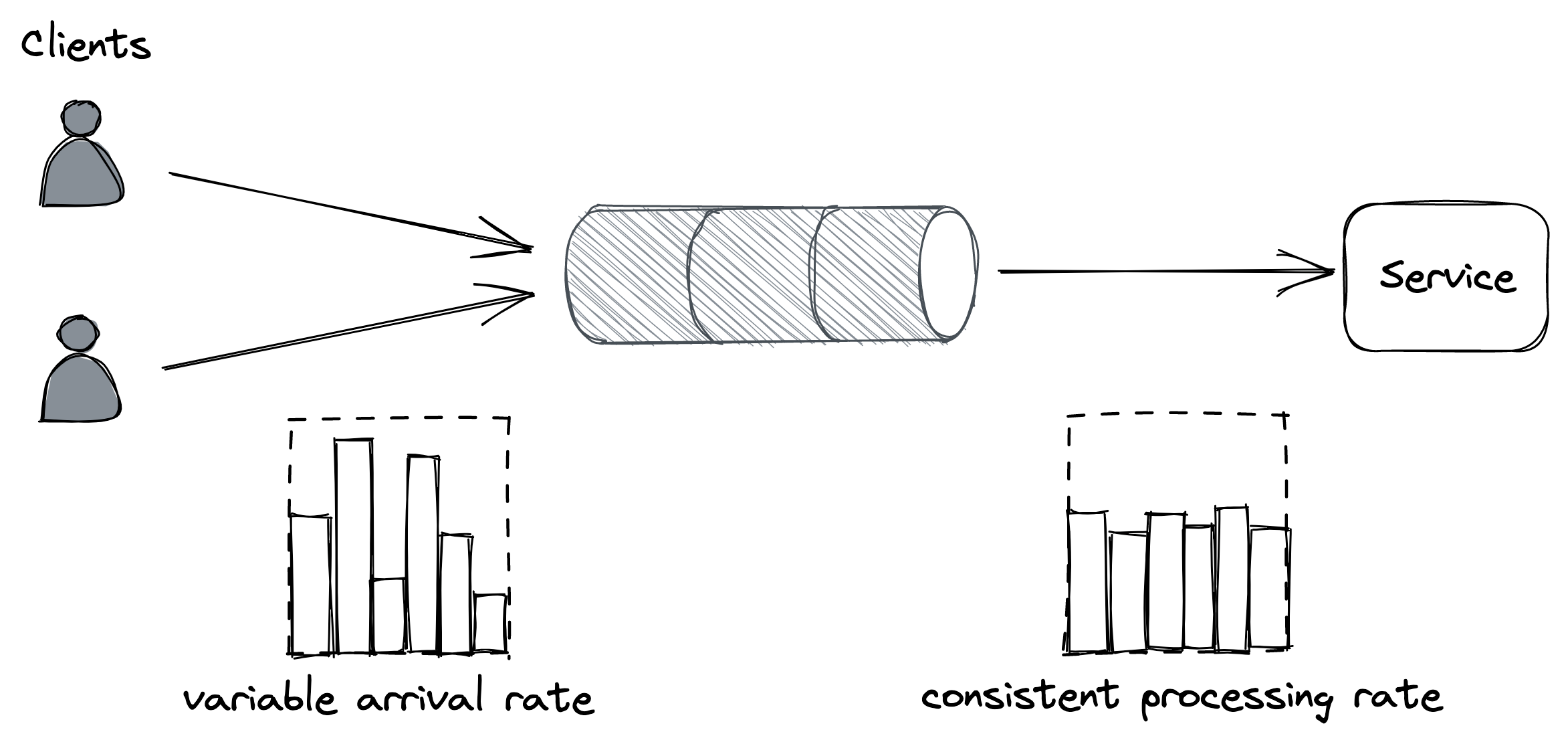
Figure 28.1: The channel smooths out the load for the consuming service.
directly but rather protect a service from getting overloaded. To handle more load, the service needs to be scaled out. This is why these protection mechanisms are typically combined with autoscaling[3], which detects that the service is running hot and automatically increases its scale to handle the additional load.
Rate-limiting
Rate-limiting, or throttling, is a mechanism that rejects a request when a specific quota is exceeded. A service can have multiple quotas, e.g., for the number of requests or bytes received within a time interval. Quotas are typically applied to specific users, API keys, or IP addresses.
For example, if a service with a quota of 10 requests per second per API key receives on average 12 requests per second from a specific API key, it will, on average, reject 2 requests per second from that API key.
When a service rate-limits a request, it needs to return a response with a particular error code so that the sender knows that it failed because a quota has been exhausted. For services with HTTP APIs, the most common way to do that is by returning a response with status code 429 (Too Many Requests). The response should include additional details about which quota has been exhausted and by how much; it can also include a Retry-After header indicating how long to wait before making a new request:
If the client application plays by the rules, it will stop hammering the service for some time, shielding the service from non-malicious users monopolizing it by mistake. In addition, this protects against bugs in the clients that cause a client to hit a downstream service for one reason or another repeatedly.
Rate-limiting is also used to enforce pricing tiers; if users want to use more resources, they should also be willing to pay more. This is how you can offload your service’s cost to your users: have them pay proportionally to their usage and enforce pricing tiers with quotas.
You would think that rate-limiting also offers strong protection against a DDoS attack, but it only partially protects a service from it. Nothing forbids throttled clients from continuing to hammer a service after getting 429s. Rate-limited requests aren’t free either — for example, to rate-limit a request by API key, the service has to pay the price of opening a TLS connection, and at the very least, download part of the request to read the key. Although rate limiting doesn’t fully protect against DDoS attacks, it does help reduce their impact.
Economies of scale are the only true protection against DDoS at-tacks. If you run multiple services behind one large gateway service, no matter which of the services behind it are attacked, the gateway service will be able to withstand the attack by rejecting the traffic upstream. The beauty of this approach is that the cost of running the gateway is amortized across all the services that are using it.
Although rate-limiting has some similarities with load shedding, they are different concepts. Load shedding rejects traffic based on the local state of a process, like the number of requests concurrently processed by it; rate-limiting instead sheds traffic based on the global state of the system, like the total number of requests concurrently processed for a specific API key across all service instances. And because there is a global state involved, some form of coordination is required.
Single-process implementation
The distributed implementation of rate-limiting is interesting in its own right, and it’s well worth spending some time discussing it. We will start with a single-process implementation first and then extend it to a distributed one.
Suppose we want to enforce a quota of 2 requests per minute, per API key. A naive approach would be to use a doubly-linked list per API key, where each list stores the timestamps of the last N requests received. Whenever a new request comes in, an entry is appended to the list with its corresponding timestamp. Then, periodically, entries older than a minute are purged from the list.
By keeping track of the list’s length, the process can rate-limit incoming requests by comparing it with the quota. The problem with this approach is that it requires a list per API key, which quickly becomes expensive in terms of memory as it grows with the number of requests received.
To reduce memory consumption, we need to come up with a way to reduce the storage requirements. One way to do this is by dividing time into buckets of fixed duration, for example of 1 minute, and keeping track of how many requests have been seen within each bucket (see Figure 28.2).
A bucket contains a numerical counter. When a new request comes in, its timestamp is used to determine the bucket it belongs to. For example, if a request arrives at 12.00.18, the counter of the bucket for minute “12.00” is incremented by 1 (see Figure 28.3).
With bucketing, we can compress the information about the number of requests seen in a way that doesn’t grow with the number of requests. Now that we have a memory-friendly representation, how can we use it to implement rate-limiting? The idea is to use a
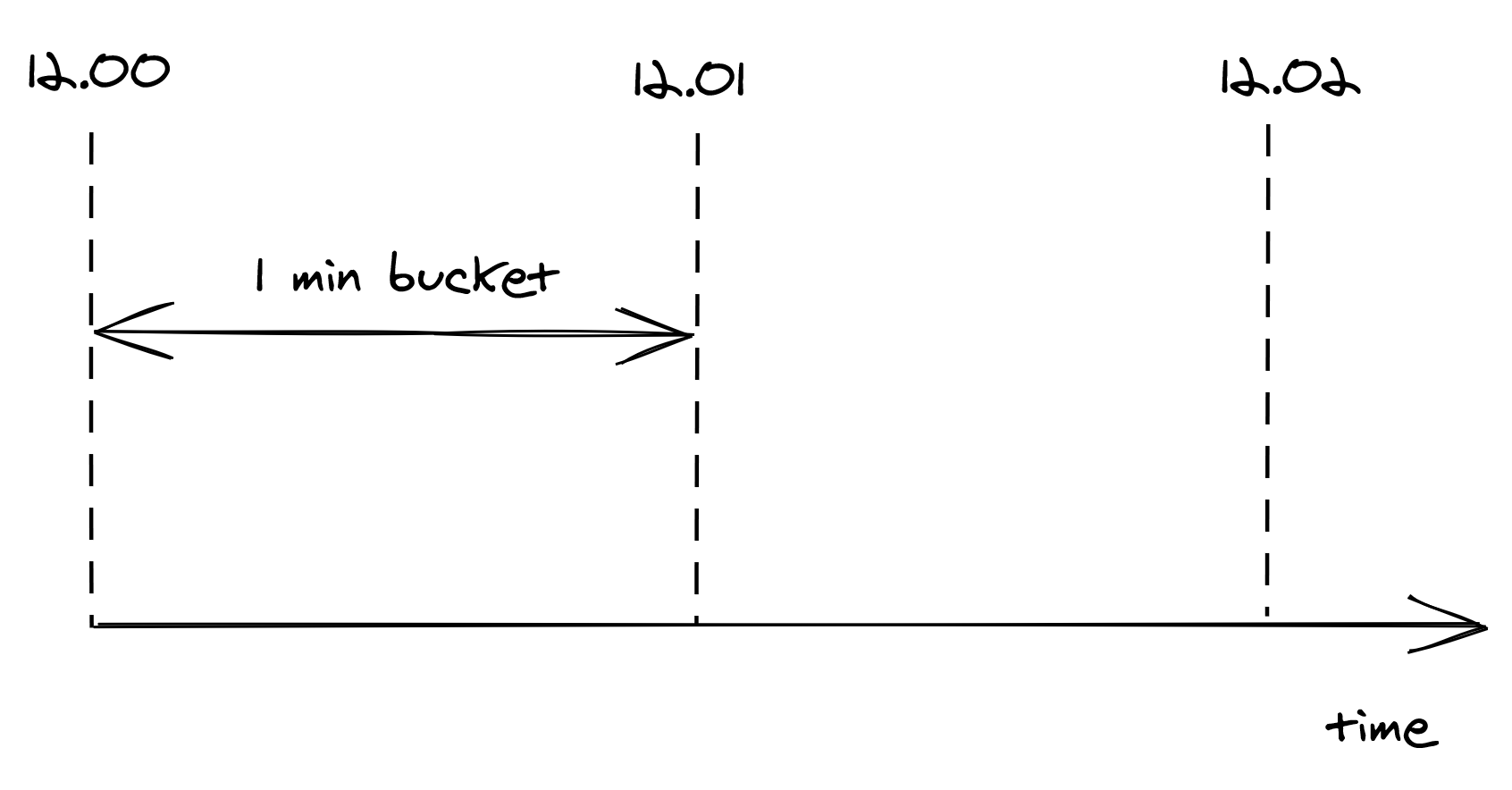
Figure 28.2: Buckets divide time into 1-minute intervals, which keep track of the number of requests seen.
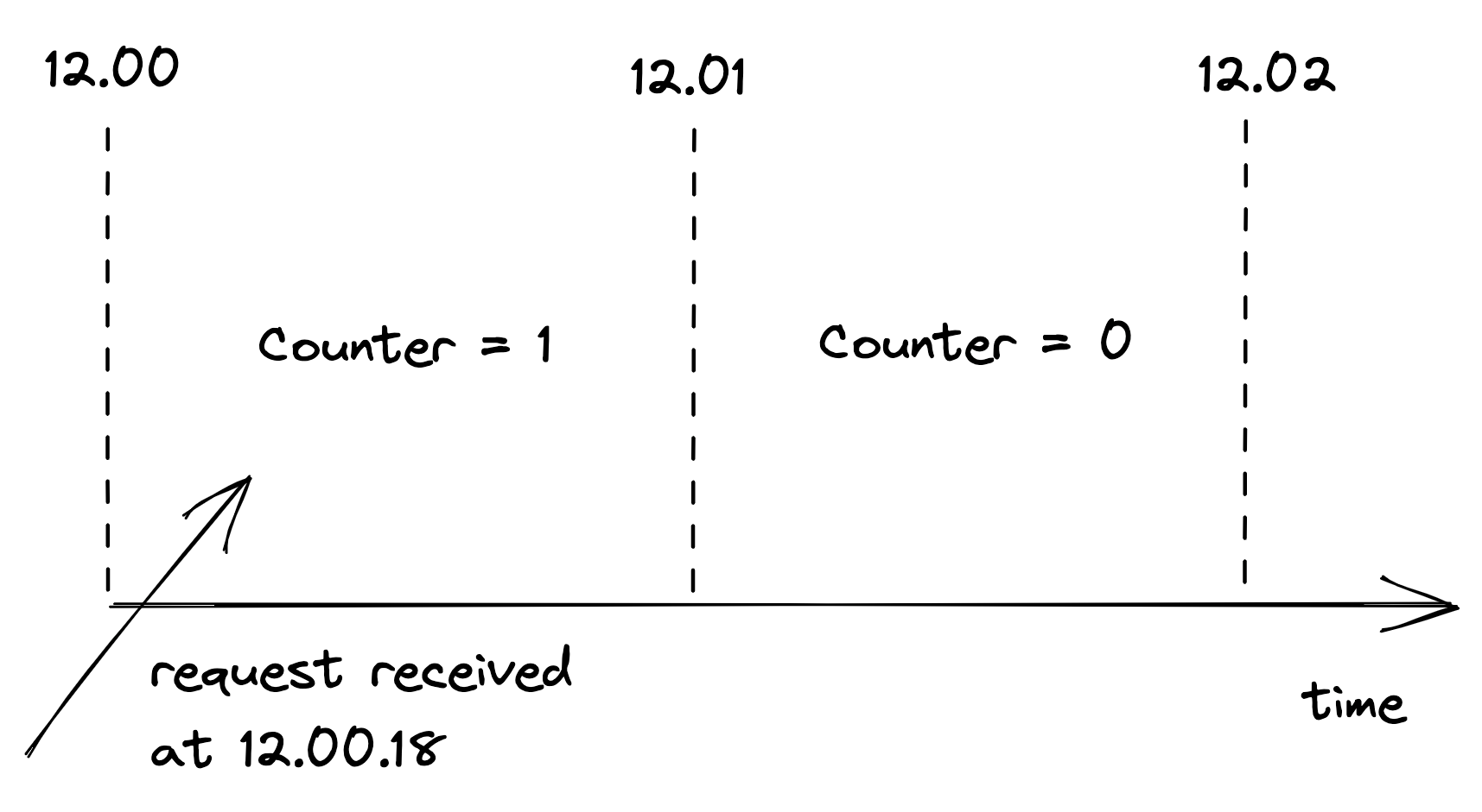
Figure 28.3: When a new request comes in, its timestamp is used to determine the bucket it belongs to.
sliding window that moves across the buckets in real time, keeping track of the number of requests within it.
The sliding window represents the interval of time used to decide whether to rate-limit or not. The window’s length depends on the time unit used to define the quota, which in our case is 1 minute. But there is a caveat: a sliding window can overlap with multiple buckets. To derive the number of requests under the sliding window, we have to compute a weighted sum of the bucket’s counters, where each bucket’s weight is proportional to its overlap with the sliding window (see Figure 28.4).
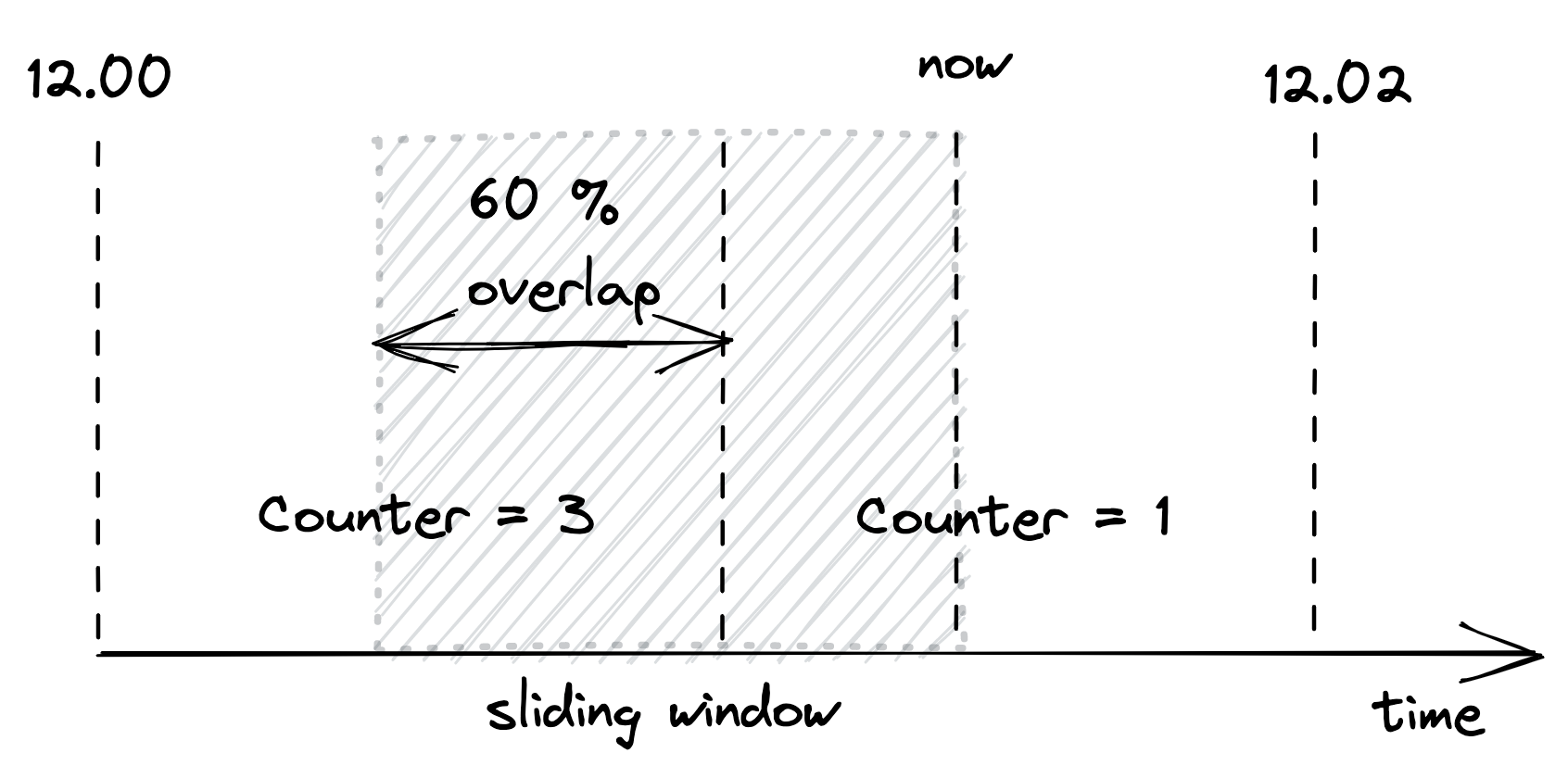
Figure 28.4: A bucket’s weight is proportional to its overlap with the sliding window.
Although this is an approximation, it’s a reasonably good one for our purposes. And it can be made more accurate by increasing the granularity of the buckets. So, for example, we can reduce the approximation error using 30-second buckets rather than 1-minute ones.
We only have to store as many buckets as the sliding window can overlap with at any given time. For example, with a 1-minute window and a 1-minute bucket length, the sliding window can overlap with at most 2 buckets. Thus, there is no point in storing the third oldest bucket, the fourth oldest one, etc.
To summarize, this approach requires two counters per API key, which is much more efficient in terms of memory than the naive implementation storing a list of requests per API key.
Distributed implementation
When more than one process accepts requests, the local state is no longer good enough, as the quota needs to be enforced on the total number of requests per API key across all service instances. This requires a shared data store to keep track of the number of requests seen.
As discussed earlier, we need to store two integers per API key, one for each bucket. When a new request comes in, the process receiving it could fetch the current bucket, update it and write it back to the data store. But that wouldn’t work because two processes could update the same bucket concurrently, which would result in a lost update. The fetch, update, and write operations need to be packaged into a single transaction to avoid any race conditions.
Although this approach is functionally correct, it’s costly. There are two issues here: transactions are slow, and executing one per request would be very expensive as the data store would have to scale linearly with the number of requests. Also, because the data store is a hard dependency, the service will become unavailable if it can’t reach it.
Let’s address these issues. Rather than using transactions, we can use a single atomic get-and-increment operation that most data stores provide. Alternatively, the same can be emulated with a compare-and-swap. These atomic operations have much better performance than transactions.
Now, rather than updating the data store on each request, the process can batch bucket updates in memory for some time and flush them asynchronously to the data store at the end of it (see Figure 28.5). This reduces the shared state’s accuracy, but it’s a good trade-off as it reduces the load on the data store and the number of requests sent to it.
What happens if the data store is down? Remember the CAP theorem’s essence: when there is a network fault, we can either sacrifice consistency and keep our system up or maintain consistency and stop serving requests. In our case, temporarily rejecting requests just because the data store used for rate-limiting is not reachable could damage the business. Instead, it’s safer to keep serving re-
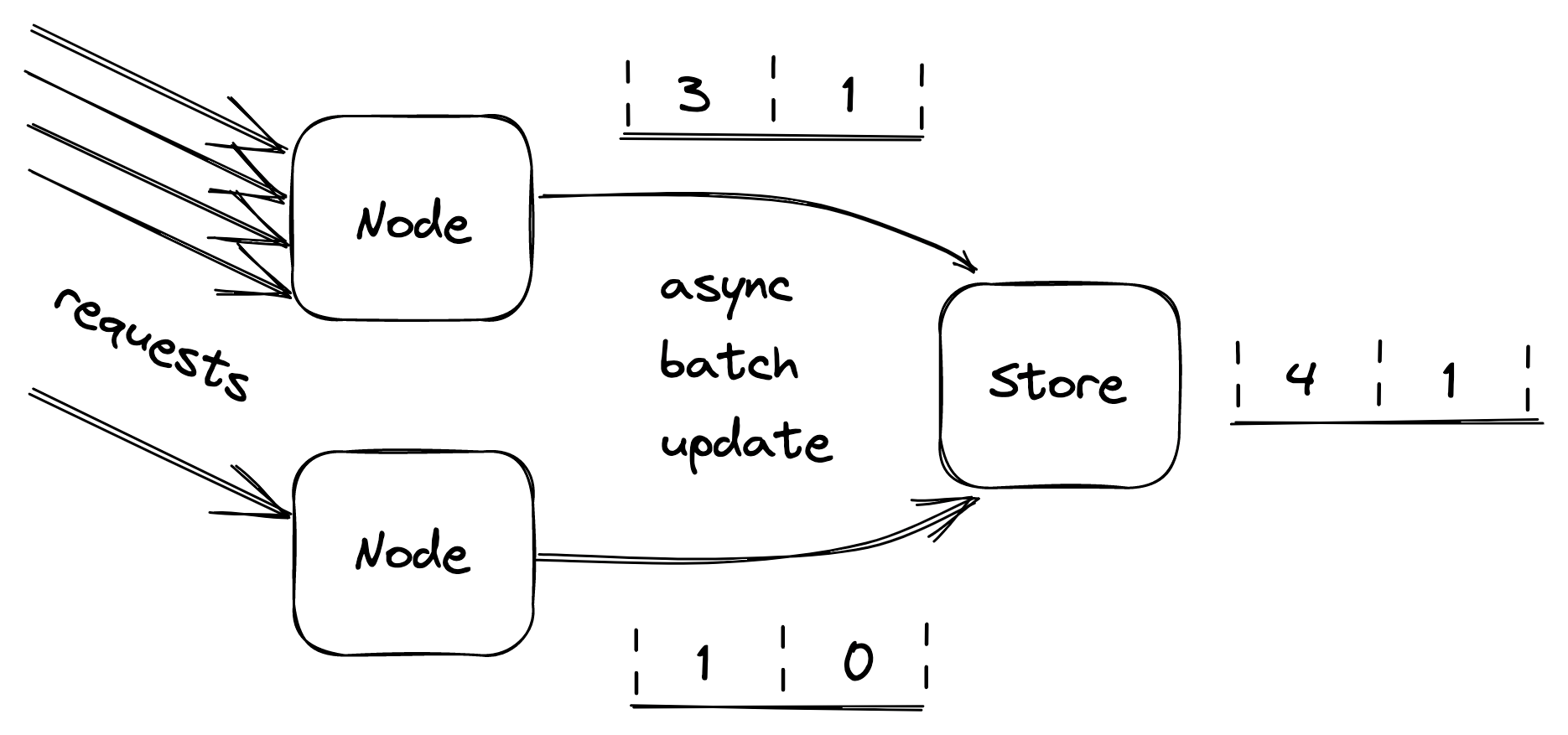
Figure 28.5: Servers batch bucket updates in memory for some time, and flush them asynchronously to the data store at the end of it.
quests based on the last state read from the store.[4]
Constant work
When overload, configuration changes, or faults force an application to behave differently from usual, we say the application has a multi-modal behavior. Some of these modes might trigger rare bugs, conflict with mechanisms that assume the happy path, and more generally make life harder for operators, since their mental model of how the application behaves is no longer valid. Thus, as a general rule of thumb, we should strive to minimize the number of modes.
For example, simple key-value stores are favored over relational databases in data planes because they tend to have predictable performance[5]. A relational database has many operational modes due to hidden optimizations, which can change how specific queries perform from one execution to another. Instead, dumb key-value stores behave predictably for a given query, which guarantees that there won’t be any surprises.
A common reason for a system to change behavior is overload, which can cause the system to become slower and degrade at the worst possible time. Ideally, the worst- and average-case behavior shouldn’t differ. One way to achieve that is by exploiting the constant work pattern, which keeps the work per unit time constant.
The idea is to have the system perform the same amount of work[6] under high load as under average load. And, if there is any variation under stress, it should be because the system is performing better, not worse. Such a system is also said to be antifragile. This is a different property from resiliency; a resilient system keeps operating under extreme load, while an antifragile one performs better.
We have already seen one application of the constant work pattern when discussing the propagation of configuration changes from the control plane to the data plane in Control planes and data planes (lesson 04.10). For example, suppose we have a configuration store (control plane) that stores a bag of settings for each user, like the quotas used by the API gateway (data plane) to rate-limit requests. When a setting changes for a specific user, the control plane needs to broadcast it to the data plane. However, as each change is a separate independent unit of work, the data plane needs to perform work proportional to the number of changes.
If you don’t see how this could be a problem, imagine that a large number of settings are updated for the majority of users at the same time (e.g., quotas changed due to a business decision). This could cause an unexpectedly large number of individual update messages to be sent to every data plane instance, which could struggle to handle them.
The workaround to this problem is simple but powerful. The control plane can periodically dump the settings of all users to a file in a scalable and highly available file store like Azure Storage or AWS S3. The dump includes the configuration settings of all users, even the ones for which there were no changes. Data plane instances can then periodically read the dump in bulk and refresh their local view of the system’s configuration. Thus, no matter how many settings change, the control plane periodically writes a file to the data store, and the data plane periodically reads it.
We can take this pattern to the extreme and pre-allocate empty configuration slots for the maximum number of supported users. This guarantees that as the number of users grows, the work required to propagate changes remains stable. Additionally, doing so allows to stress-test the system and understand its behavior, knowing that it will behave the same under all circumstances. Although this limits the number of users, a limit exists regardless of whether the constant work pattern is used or not. This approach is typically used in cellular architectures (see 26.2), where a single cell has a well-defined maximum size and the system is scaled out by creating new cells.
The beauty of using the constant work pattern is that the data plane periodically performs the same amount of work in bulk, no matter how many configuration settings have changed. This makes updating settings reliable and predictable. Also, periodically writing and reading a large file is much simpler to implement correctly than a complex mechanism that only sends what changed.
Another advantage of this approach is that it’s robust against a whole variety of faults thanks to its self-healing properties. If the configuration dump gets corrupted for whatever reason, no harm is done since the next update will fix it. And if a faulty update was pushed to all users by mistake, reverting it is as simple as creating a new dump and waiting it out. In contrast, the solution that sends individual updates is much harder to implement correctly, as the data plane needs complex logic to handle and heal from corrupted updates.
To sum up, performing constant work is more expensive than doing just the necessary work. Still, it’s often worth considering it, given the increase in reliability and reduction in complexity it enables.
As the number of components or operations in a system increases, so does the number of failures, and eventually, anything that can happen will happen. In my team, we humorously refer to this as “cruel math.”
If you talk to an engineer responsible for a production system, you will quickly realize that they tend to be more worried about minimizing and tolerating failures than how to further scale out their systems. The reason for that is that once you have an architecture that scales to handle your current load, you will be mostly concerned with tolerating faults until you eventually reach the next scalability bottleneck.
What you should take away from this part is that failures are inevitable since, no matter how hard you try, it’s just impossible to build an infallible system. When you can’t design away some failure modes (e.g., with constant work), the best you can do is to reduce their blast radius and stop the cracks from propagating from one component to the other.
Module references
References
- Also known as Murphy’s law
References
- “A Conceptual Framework for System Fault Tolerance,” https://resources.sei.cmu.edu/asset_files/TechnicalReport/1992_005_001_16112.pdf
- “Simple Testing Can Prevent Most Critical Failures: An Analysis of Production Failures in Distributed Data-Intensive Systems,” https://www.usenix.org/system/files/conference/osdi14/osdi14-paper-yuan.pdf
- This is the reason the Go language puts so much emphasis on error handling.
- “A List of Post-mortems: Config Errors,” https://github.com/danluu/post-mortems#config-errors
- “Early Detection of Configuration Errors to Reduce Failure Damage,” https://www.usenix.org/system/files/conference/osdi16/osdi16-xu.pdf
- “It’s always DNS,” https://twitter.com/ahidalgosre/status/1315345619926609920?lang=en-GB
- “Foursquare Goes Dark Too. Unintentionally.,” https://techcrunch.com/2010/03/27/foursquare-offline
- “Stop using .IO Domain Names for Production Traffic,” https://hackernoon.com/stop-using-io-domain-names-for-production-traffic-b6aa17eeac20
- “Microsoft Teams goes down after Microsoft forgot to renew a certificate,” https://www.theverge.com/2020/2/3/21120248/microsoft-teams-down-outage-certificate-issue-status
- “Fallacies of distributed computing,” https://en.wikipedia.org/wiki/Fallacies_of_distributed_computing
- “Gray Failure: The Achilles’ Heel of Cloud-Scale Systems,” https://www.microsoft.com/en-us/research/wp-content/uploads/2017/06/paper-1.pdf
- “Metastable Failures in Distributed Systems,” https://sigops.org/s/conferences/hotos/2021/papers/hotos21-s11-bronson.pdf
- “Risk matrix,” https://en.wikipedia.org/wiki/Risk_matrix
References
- “When Redundancy Actually Helps,” https://brooker.co.za/blog/2019/06/20/redundancy.html
- “Active-Active for Multi-Regional Resiliency,” https://netflixtechblog.com/active-active-for-multi-regional-resiliency-c47719f6685b
- “The CJEU judgment in the Schrems II case,” https://www.europarl.europa.eu/RegData/etudes/ATAG/2020/652073/EPRS_ATA(2020)652073_EN.pdf
References
- We discussed partitioning in Partitioning (lesson 04.04) from a scalability point of view.
- “Shuffle Sharding: Massive and Magical Fault Isolation,” https://aws.amazon.com/blogs/architecture/shuffle-sharding-massive-and-magical-fault-isolation/
- Partitioning by user is just an example; we could partition just as well by physical location, workload, or any other dimension that makes sense for the application.
- “New Relic case: Huge scale, small clusters: Using Cells to scale in the Cloud,” https://www.youtube.com/watch?v=eMikCXiBlOA
References
- “Web APIs: XMLHttpRequest.timeout,” https://developer.mozilla.org/en-US/docs/Web/API/XMLHttpRequest/timeout
- “Add a timeout option, to prevent hanging,” https://github.com/whatwg/fetch/issues/951
- “Web APIs: AbortController,” https://developer.mozilla.org/en-US/docs/Web/API/AbortController
- “Requests Quickstart: Timeouts,” https://requests.readthedocs.io/en/master/user/quickstart/#timeouts
- “net/http: make default configs have better timeouts,” https://github.com/golang/go/issues/24138
- “HttpClient.Timeout Property,” https://docs.microsoft.com/en-us/dotnet/api/system.net.http.httpclient.timeout?view=net-6.0#remarks
- “Timeouts, retries, and backoff with jitter,” https://aws.amazon.com/builders-library/timeouts-retries-and-backoff-with-jitter/
- “Exponential Backoff And Jitter,” https://aws.amazon.com/blogs/architecture/exponential-backoff-and-jitter/
References
- We have already met a mechanism to protect against upstream pressure when we discussed health checks in the context of load balancers in Network load balancing (lesson 04.06).
- “Using load shedding to avoid overload,” https://aws.amazon.com/builders-library/using-load-shedding-to-avoid-overload
- “Autoscaling,” https://en.wikipedia.org/wiki/Autoscaling
- This is another application of the concept of static stability, first introduced in Control planes and data planes (lesson 04.10).
- “Some opinionated thoughts on SQL databases,” https://blog.nelhage.com/post/some-opinionated-sql-takes/
- “Reliability, constant work, and a good cup of coffee,” https://aws.amazon.com/builders-library/reliability-and-constant-work/