Study one concept at a time. Open the guided module →
Maintainability
Overview: Maintainability
Video coming soon. Start with the reading below.
“Everyone knows that debugging is twice as hard as writing a program in the first place. So if you’re as clever as you can be when you write it, how will you ever debug it?”
– Brian Kernighan
It’s a well-known fact that the majority of the cost of software is spent after its initial development in maintenance activities, such as fixing bugs, adding new features, and operating it. Thus, we should aspire to make our systems easy to modify, extend and operate so that they are easy to maintain.
Good testing — in the form of unit, integration, and end-to-end tests — is a minimum requirement to be able to modify or extend a system without worrying it will break. And once a change has been merged into the codebase, it needs to be released to production safely without affecting the application’s availability. Also, the operators need to be able to monitor the system’s health, investigate degradations and restore the service when it gets into a bad state. This requires altering the system’s behavior without code changes, e.g., toggling a feature flag or scaling out a service with a configuration change.
Historically, developers, testers, and operators were part of different teams. First, the developers handed over their software to a team of QA engineers responsible for testing it. Then, when the software passed that stage, it moved to an operations team responsible for deploying it to production, monitoring it, and responding to alerts. However, this model is being phased out in the industry. Nowadays, it’s common for developers to be responsible for testing and operating the software they write, which requires embracing an end-to-end view of the software’s lifecycle.
In this part, we will explore some of the best practices for testing and operating large distributed applications.
Testing (lesson 06.02) describes the different types of tests — unit, integration, and end-to-end tests — that we can leverage to increase the confidence that a distributed application works as expected. This lesson also explores the use of formal verification methods to verify the correctness of an application before writing a single line of code.
Continuous delivery and deployment (lesson 06.03) dives into continuous delivery and deployment pipelines to release changes safely and efficiently to production.
Monitoring (lesson 06.04) discusses how to use metrics, service-level indicators, and dashboards to monitor the health of distributed applications. It then talks about how to define and enforce service-level objectives that describe how the service should behave when it’s functioning correctly.
Observability (lesson 06.05) introduces the concept of observability and its relation to monitoring. Later, it describes how to debug production issues using logs and traces.
Manageability (lesson 06.06) describes how to modify a system’s behavior without changing its code, which is a must-have to enable operators to quickly mitigate failures in production when everything else fails.
Testing
Video coming soon. Start with the reading below.
The longer it takes to detect a bug, the more expensive it becomes to fix. A software test can verify that some part of the application works as intended, catching bugs early in the process. But the real benefit that comes from testing shows up only later when developers want to make changes to the existing implementation (e.g., bug fixes, refactorings, and new features) without breaking the expected behaviors. Tests also act as always up-to-date documentation and improve the quality of public interfaces since developers have to put themselves in the users’ shoes to test them effectively.
Unfortunately, testing is not a silver bullet because it’s impossible to predict all the states a complex distributed application can get into. It only provides best-effort guarantees that the code being tested is correct and fault-tolerant. No matter how exhaustive the test coverage is, tests can only cover failures developers can imagine, not the kind of complex emergent behavior that manifests itself in production[1].
Although tests can’t guarantee that code is bug-free, they certainly do a good job validating expected behaviors. So, as a rule of thumb, if you want to be confident that your implementation behaves in a certain way, you have to add a test for it.
Scope
Tests come in different shapes and sizes. To begin with, we need to distinguish between the code paths a test is actually testing (aka system under test or SUT) from the ones that are being run. The SUT represents the scope of the test. It determines whether the test is categorized as a unit test, an integration test, or an end-to-end test.
A unit test validates the behavior of a small part of the codebase, like an individual class[2]. A good unit test should be relatively static in time and change only when the behavior of the SUT changes — refactoring, bug fixes, or new features shouldn’t break it. To achieve that, a unit test should:
- use only the public interfaces of the SUT;
- test for state changes in the SUT (not predetermined sequences of actions);
- test for behaviors, i.e., how the SUT handles a given input when it’s in a specific state.
An integration test has a larger scope than a unit test, since it verifies that a service can interact with an external dependency as expected. Confusingly, integration testing has different meanings for different people. Martin Fowler[3] makes the distinction between narrow and broad integration tests. A narrow integration test exercises only the code paths of a service that communicate with a specific external dependency, like an adapter and its supporting classes. In contrast, a broad integration test exercises code paths across multiple live services. In the rest of the chapter, we will refer to these broader integration tests as end-to-end tests.
An end-to-end test validates behavior that spans multiple services in the system, like a user-facing scenario. These tests usually run in shared environments, like staging or production, and therefore should not impact other tests or users sharing the same environment. Because of their scope, they are slow and more prone to intermittent failures.
End-to-end tests can also be painful and expensive to maintain. For example, when an end-to-end test fails, it’s generally not obvious which service caused the failure, and a deeper investigation is required. But these tests are a necessary evil to ensure that userfacing scenarios work as expected across the entire application. They can uncover issues that tests with smaller scope can’t, like unanticipated side effects and emergent behaviors.
One way to minimize the number of end-to-end tests is to frame them as user journey tests. A user journey test simulates a multi-step interaction of a user with the system (e.g., for an e-commerce service: create an order, modify it, and finally cancel it). Such a test usually requires less time to run than the individual journey parts split into separate end-to-end tests.
As the scope of a test increases, it becomes more brittle, slow, and costly. Intermittently failing tests are nearly as bad as no tests at all, as developers stop trusting them and eventually ignore their failures. When possible, it’s preferable to have tests with smaller scope as they tend to be more reliable, faster, and cheaper. A good trade-off is to have a large number of unit tests, a smaller fraction of integration tests, and even fewer end-to-end tests (see Figure 29.1).
Size
The size of a test[4] reflects how much computing resources it needs to run, like the number of nodes. Generally, that depends on how realistic the environment is where the test runs. Although
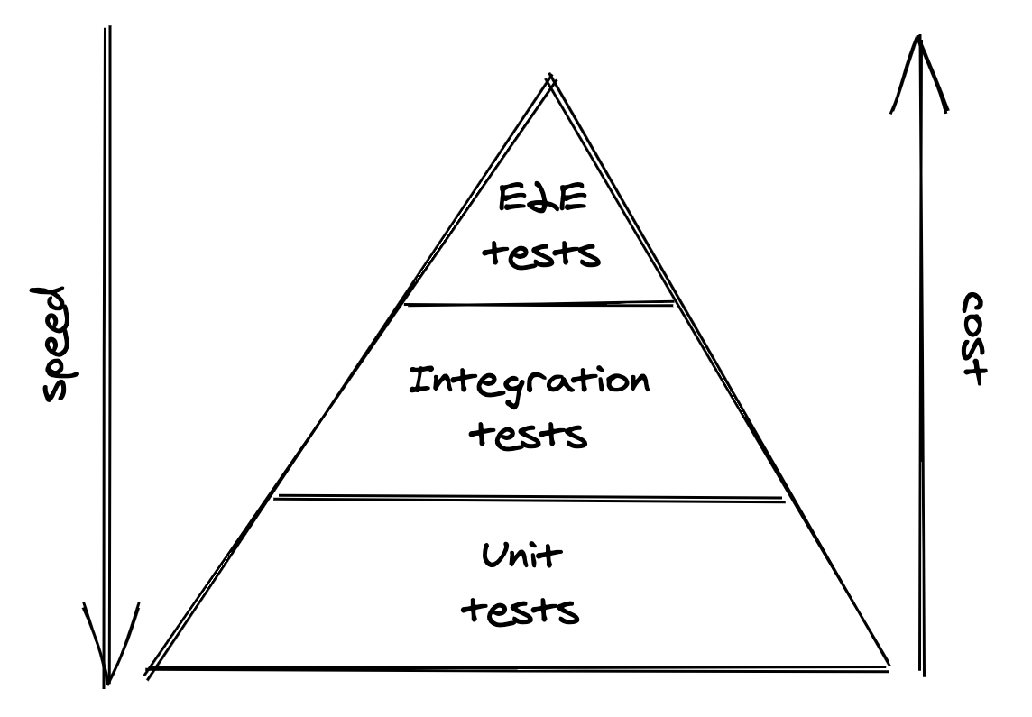
Figure 29.1: Test pyramid
the scope and size of a test tend to be correlated, they are distinct concepts, and it helps to separate them.
A small test runs in a single process and doesn’t perform any blocking calls or I/O. As a result, it’s very fast, deterministic, and has a very small probability of failing intermittently.
An intermediate test runs on a single node and performs local I/O, like reads from disk or network calls to localhost. This introduces more room for delays and non-determinism, increasing the likelihood of intermittent failures.
A large test requires multiple nodes to run, introducing even more non-determinism and longer delays.
Unsurprisingly, the larger a test is, the longer it takes to run and the flakier it becomes. This is why we should write the smallest possible test for a given behavior. We can use a test double in place of a real dependency, such as a fake, a stub, or a mock, to reduce the test’s size, making it faster and less prone to intermittent failures:
- A fake is a lightweight implementation of an interface that behaves similarly to a real one. For example, an in-memory version of a database is a fake.
- A stub is a function that always returns the same value no
matter which arguments are passed to it. • Finally, a mock has expectations on how it should be called, and it’s used to test the interactions between objects.
The problem with test doubles is that they don’t resemble how the real implementation behaves with all its nuances. The weaker the resemblance is, the less confidence we should have that the test using the double is actually useful. Therefore, when the real implementation is fast, deterministic, and has few dependencies, we should use that rather than a double. When using the real implementation is not an option, we can use a fake maintained by the same developers of the dependency if one is available. Stubbing, or mocking, are last-resort options as they offer the least resemblance to the actual implementation, which makes tests that use them brittle.
For integration tests, a good compromise is to combine mocking with contract tests[5]. A contract test defines a request for an external dependency with the corresponding expected response. Then the test uses this contract to mock the dependency. For example, a contract for a REST API consists of an HTTP request and response. To ensure that the contract is valid and doesn’t break in the future, the test suite of the external dependency uses the same contract definition to simulate the client request and ensure that the expected response is returned.
Practical considerations
As with everything else, testing requires making trade-offs. Suppose we want to end-to-end test the behavior of a specific API end-point exposed by a service. The service talks to:
- a data store,
- an internal service owned by another team,
- and a third-party API used for billing (see Figure 29.2).
As suggested earlier, we should try to write the smallest possible test for the desired scope while minimizing the use of test doubles that don’t resemble how the real implementation behaves.
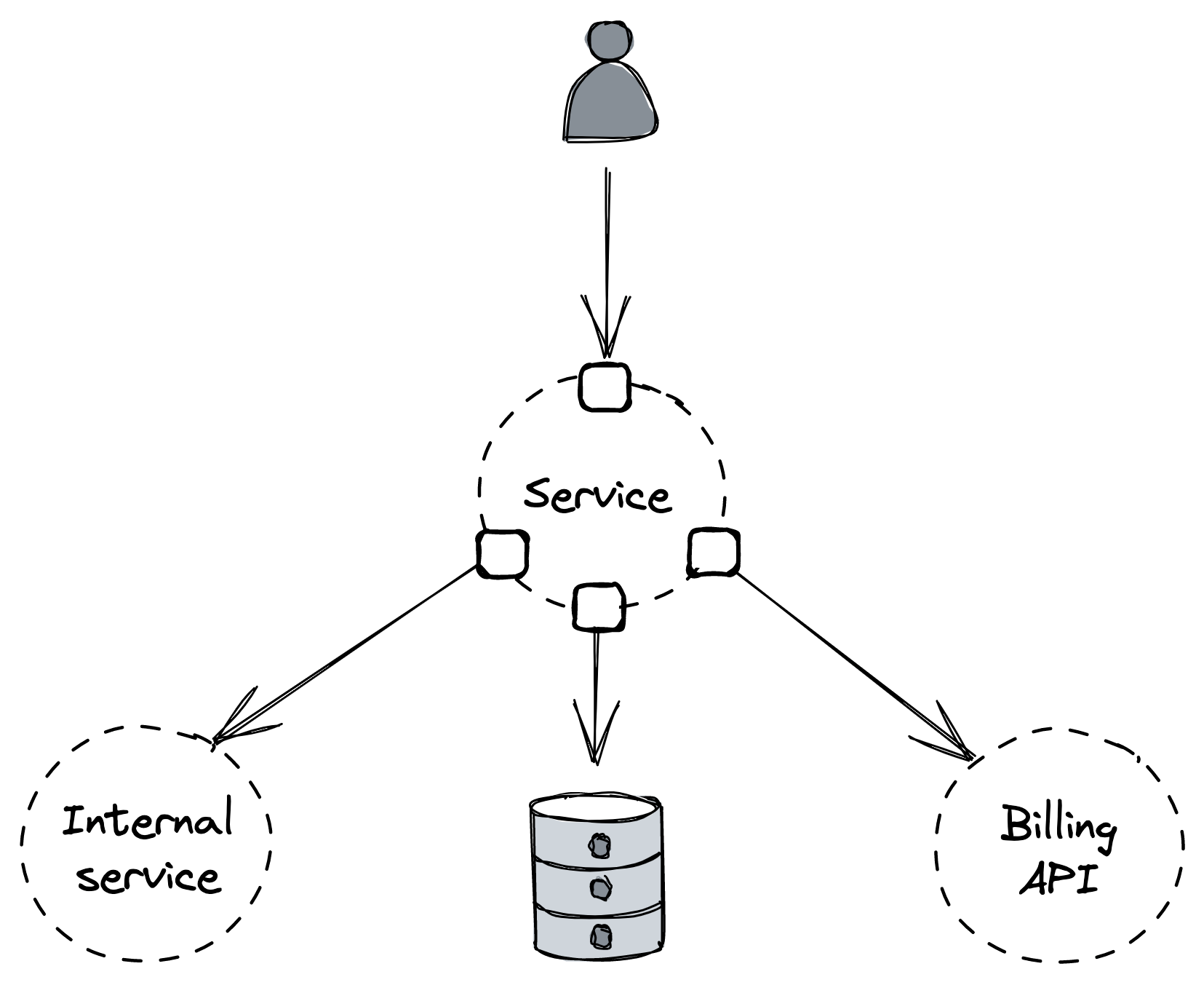
Figure 29.2: How should we test the service?
Let’s assume the specific endpoint under test doesn’t communicate with the internal service, so we can safely use a mock in its place. And if the data store comes with an in-memory implementation (a fake), we can use that in the test to avoid issuing network calls. Finally, we can’t easily call the third-party billing API since that would require issuing real transactions. However, assuming a fake is not available, the billing service might still offer a testing endpoint that issues fake transactions.
Here is a more nuanced example in which it’s a lot riskier to go for a smaller test. Suppose we need to test whether purging the data belonging to a specific user across the entire application stack works as expected. In Europe, this functionality is mandated by law (GDPR), and failing to comply with it can result in fines up to 20 million euros or 4% annual turnover, whichever is greater. In this case, because the risk of the functionality silently breaking is high, we want to be as confident as possible that it’s working as expected. This warrants the use of an end-to-end test that runs in production periodically and uses live services rather than test doubles.
Formal verification
Software tests are not the only way to catch bugs early. Taking the time to write a high-level description of how a system behaves, i.e., a specification, allows subtle bugs and architecture shortcomings to be detected before writing a single line of code.
A specification can range from an informal one-pager to a formal mathematical description that a computer can check. Since it’s hard to specify what we don’t fully understand, a specification can help us reason about the behaviors of the system we are designing. It also acts as documentation for others and as a guide for the actual implementation. On top of the benefits mentioned so far, by writing the specification in a formal language, we also gain the ability to verify algorithmically whether the specification is flawed (model checking).
Writing a specification doesn’t mean describing every corner of a system in detail. The specification’s goal is to catch errors while they are still cheap to fix. Therefore, we only want to specify those parts that are most likely to contain errors and are hard to detect by other means, like traditional tests. Once we have decided what to specify, we also need to choose the level of abstraction, i.e., which details to omit.
TLA+[6] is a well-known and widely used formal specification language[7]. The likes of Amazon or Microsoft use it to describe some of their most complex distributed systems, like S3 or Cosmos DB[8].
In TLA+, a behavior of a system is represented by a sequence of states, where a state is an assignment of values to global variables.
Thus, the specification of a system is the set of all possible behaviors.
One of the goals of writing a specification is to verify that it satisfies properties we want the system to have, like safety and liveness. A safety property asserts that something is true for all states of a behavior (invariant). A liveness property instead asserts that something eventually happens. TLA+ allows to describe and verify properties that should be satisfied by all possible states and behaviors of a specification. This is extremely powerful, since a system running at scale will eventually run into all possible states and behaviors, and humans are bad at imagining behaviors in which several rare events occur simultaneously.
For example, suppose we have a service that uses key-value store X, and we would like to migrate it to use key-value store Y that costs less and has proven to perform better in benchmarks. At a high level, one way we could implement this migration without any downtime is the following:
- The service writes to both data stores X and Y (dual write) while reading exclusively from X.
- A one-off batch process backfills Y with data from X created before the service started writing to Y.
- The application switches to read and write exclusively from and to Y.
This approach might seem reasonable, but will it guarantee that the data stores eventually end up in the same state?
If we were to model this with TLA+, the model checker would be able to identify several problems, like a liveness violation that leaves the system in an inconsistent state when a service instance crashes after writing to A but before writing to B. The beauty of automated model checking is that it returns an error trace with the behavior (i.e., sequence of states) that violates the properties when it fails.
Although modeling writes as atomic (i.e., either both writes succeed, or they both fail) fixes the liveness issue, the model isn’t correct yet. For example, if two service instances are writing to A and B simultaneously, the two data stores can end up in different states because the order of writes can differ, as shown in Fig 29.3.
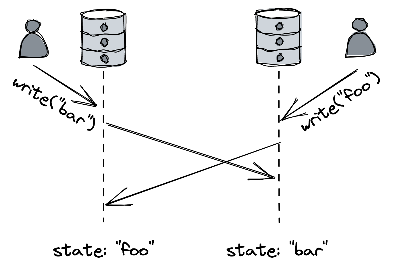
Figure 29.3: Data stores can see writes in different orders.
If you remember the discussion about transactions in Outbox pattern in Asynchronous transactions, you know we can solve this problem by introducing a message channel between the service and data stores that serializes all writes and guarantees a single global order. Regardless of the actual solution, the point is that a formal model enables us to test architectural decisions that would be hard to verify otherwise.
Continuous delivery and deployment
Video coming soon. Start with the reading below.
Once a change and its newly introduced tests have been merged to a repository, it needs to be released to production. When releasing a change requires a manual process, it won’t happen frequently. This means that several changes, possibly over days or even weeks, end up being batched and released together, increasing the likelihood of the release failing. And when a release fails, it’s harder to pinpoint the breaking change[1], slowing down the team. Also, the developer who initiated the release needs to keep an eye on it by monitoring dashboards and alerts to ensure that it’s working as expected or roll it back.
Manual deployments are a terrible use of engineering time. The problem gets further exacerbated when there are many services. Eventually, the only way to release changes safely and efficiently is to automate the entire process. Once a change has been merged to a repository, it should automatically be rolled out to production safely. The developer is then free to context-switch to their next task rather than shepherding the deployment. The whole release process, including rollbacks, can be automated with a continuous delivery and deployment (CD) pipeline.
Because releasing changes is one of the main sources of failures, CD requires a significant amount of investment in terms of safeguards, monitoring, and automation. If a regression is detected, the artifact being released — i.e., the deployable component that includes the change — is either rolled back to the previous version or forward to the next one, assuming it contains a hotfix.
There is a balance between the safety of a rollout and the time it takes to release a change to production. A good CD pipeline should strive to make a good trade-off between the two. In this lesson, we will explore how.
Review and build
At a high level, a code change needs to go through a pipeline of four stages to be released to production: review, build, pre-production rollout, and production rollout.
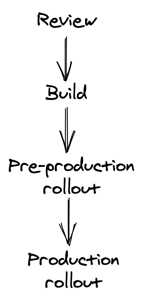
Figure 30.1: Continuous delivery and deployment pipeline stages
It all starts with a pull request (PR) submitted for review by a developer to a repository. When the PR is submitted for review, it needs to be compiled, statically analyzed, and validated with a battery of tests, all of which shouldn’t take longer than a few minutes. To increase the tests’ speed and minimize intermittent failures, the tests that run at this stage should be small enough to run on a single process or node, while larger tests run later in the pipeline.
The PR needs to be reviewed and approved by a team member before it can be merged into the repository. The reviewer has to validate whether the change is correct and safe to be released to production automatically by the CD pipeline. A checklist can help the reviewer not to forget anything important, e.g.:
- Does the change include unit, integration, and end-to-end tests as needed?
- Does the change include metrics, logs, and traces?
- Can this change break production by introducing a backward-incompatible change or hitting some service limit?
- Can the change be rolled back safely, if needed?
Code changes shouldn’t be the only ones going through this review process. For example, static assets, end-to-end tests, and configuration files should all be version-controlled in a repository (not necessarily the same one) and be treated just like code. The same service can then have multiple CD pipelines, one for each repository, potentially running in parallel.
I can’t stress enough the importance of reviewing and releasing configuration changes with a CD pipeline. As discussed in Common failure causes (lesson 05.02), one of the most common causes of production failures are configuration changes applied globally without any prior review or testing.
Also, applications running in the cloud should declare their infrastructure dependencies, like virtual machines, data stores, and load balancers, with code (aka Infrastructure as Code (IaC)[2]) using tools like Terraform[3]. This allows the provisioning of infrastructure to be automated and infrastructure changes to be treated just like any other software change.
Once a change has been merged into its repository’s main branch, the CD pipeline moves to the build stage, in which the repository’s content is built and packaged into a deployable release artifact.
Pre-production
During this stage, the artifact is deployed and released to a synthetic pre-production environment. Although this environment lacks the realism of production, it’s useful to verify that no hard failures are triggered (e.g., a null pointer exception at startup due to a missing configuration setting) and that end-to-end tests succeed. Because releasing a new version to pre-production requires significantly less time than releasing it to production, bugs can be detected earlier.
There can be multiple pre-production environments, starting with one created from scratch for each artifact and used to run simple smoke tests, to a persistent one similar to production that receives a small fraction of mirrored requests from it. AWS, for example, is known for using multiple pre-production environments[4].
Ideally, the CD pipeline should assess the artifact’s health in pre-production using the same health signals used in production. Metrics, alerts, and tests used in pre-production should be equivalent to those used in production, to avoid the former becoming a second-class citizen with sub-par health coverage.
Production
Once an artifact has been rolled out to pre-production successfully, the CD pipeline can proceed to the final stage and release the artifact to production. It should start by releasing it to a small number of production instances at first[5]. The goal is to surface problems that haven’t been detected so far as quickly as possible before they have the chance to cause widespread damage in production.
If that goes well and all the health checks pass, the artifact is incrementally released to the rest of the fleet. While the rollout is in progress, a fraction of the fleet can’t serve any traffic due to the ongoing deployment, and so the remaining instances need to pick up the slack. For this to not cause any performance degradation, there needs to be enough capacity left to sustain the incremental release.
If the service is available in multiple regions, the CD pipeline should first start with a low-traffic region to reduce the impact of a faulty release. Then, releasing the remaining regions should be divided into sequential stages to minimize risks further. Naturally, the more stages there are, the longer the CD pipeline takes to release the artifact to production. One way to mitigate this problem is by increasing the release speed once the early stages complete successfully and enough confidence has been built up. For example, the first stage could release the artifact to a single region, the second to a larger region, and the third to N regions simultaneously.
Rollbacks
After each step, the CD pipeline needs to assess whether the artifact deployed is healthy and, if not, stop the release and roll it back. A variety of health signals can be used to make that decision, such as the result of end-to-end tests, health metrics like latencies and errors and alerts.
Monitoring just the health signals of the service being rolled out is not enough. The CD pipeline should also monitor the health of upstream and downstream services to detect any indirect impact of the rollout. The pipeline should allow enough time to pass between one step and the next (bake time) to ensure that it was successful, as some issues only appear after some time has passed. For example, a performance degradation could be visible only at peak time. To speed up the release, the bake time can be reduced after each step succeeds and confidence is built up. The CD pipeline could also gate the bake time on the number of requests seen for specific API endpoints to guarantee that the API surface has been properly exercised.
When a health signal reports a degradation, the CD pipeline stops. At that point, it can either roll back the artifact automatically or trigger an alert to engage the engineer on call, who needs to decide whether a rollback is warranted or not[6]. Based on the engineer’s input, the CD pipeline retries the stage that failed (e.g., perhaps because something else was going into production at the time) or rolls back the release entirely.
The operator can also stop the pipeline and wait for a new artifact with a hotfix to be rolled forward. This might be necessary if the release can’t be rolled back because of a backward-incompatible change. Since rolling forward is much riskier than rolling back, any change introduced should always be backward compatible as a rule of thumb. One of the most common causes for backward incompatibility is changing the serialization format used for persistence or IPC purposes.
To safely introduce a backward-incompatible change, it needs to be broken down into multiple backward-compatible changes[7]. For example, suppose the messaging schema between a producer and a consumer service needs to change in a backward-incompatible way. In this case, the change is broken down into three smaller changes that can individually be rolled back safely:
- In the prepare change, the consumer is modified to support both the new and old messaging format.
- In the activate change, the producer is modified to write the messages in the new format.
- Finally, in the cleanup change, the consumer stops supporting the old messaging format altogether. This change is only released once there is enough confidence that the activated change won’t need to be rolled back.
An automated upgrade-downgrade test part of the CD pipeline in pre-production can be used to validate whether a change is actually safe to roll back.
Monitoring
Video coming soon. Start with the reading below.
Monitoring is primarily used to detect failures that impact users in production and to trigger notifications (or alerts) to the human operators responsible for the system. Another important use case for monitoring is to provide a high-level overview of the system’s health via dashboards.
In the early days, monitoring was used mostly to report whether a service was up, without much visibility of what was going on inside (black-box monitoring). In time, developers also started to instrument their applications to report whether specific features worked as expected (white-box monitoring). This was popularized with the introduction of statsd[1] by Etsy, which normalized collecting application-level measurements. While black-box monitoring is useful for detecting the symptoms of a failure, white-box monitoring can help identify the root cause.
The main use case for black-box monitoring is to monitor external dependencies, such as third-party APIs, and validate how users perceive the performance and health of a service from the outside. A common black-box approach is to periodically run scripts (synthetics[2]) that send test requests to external API endpoints and monitor how long they took and whether they were successful. Synthetics are deployed in the same regions the application’s users are and hit the same endpoints they do. Because they exercise the system’s public surface from the outside, they can catch issues that aren’t visible from within the application, like connectivity problems. Synthetics are also useful for detecting issues with APIs that aren’t exercised often by users.
For example, if the DNS server of a service were down, the issue would be visible to synthetics, since they wouldn’t be able to resolve its IP address. However, the service itself would think everything was fine, and it was just getting fewer requests than usual.
Metrics
A metric is a time series of raw measurements (samples) of resource usage (e.g., CPU utilization) or behavior (e.g., number of requests that failed), where each sample is represented by a floating-point number and a timestamp.
Commonly, a metric can also be tagged with a set of key-value pairs (labels). For example, the label could represent the region, data center, cluster, or node where the service is running. Labels make it easy to slice and dice the data and eliminate the instrumentation cost of manually creating a metric for each label combination. However, because every distinct combination of labels is a different metric, tagging generates a large number of metrics, making them challenging to store and process.
At the very least, a service should emit metrics about its load (e.g., request throughput), its internal state (e.g., in-memory cache size), and its dependencies’ availability and performance (e.g., data store response time). Combined with the metrics emitted by downstream services, this allows operators to identify problems quickly. But this requires explicit code changes and a deliberate effort by developers to instrument their code.
For example, take a fictitious HTTP handler that returns a resource. There is a whole range of questions we will want to be able to answer once it’s running in production[3]:
def get_resource(id):
  resource = self._cache.get(id)
                                  # in-process cache
  # Is the id valid?
  # Was there a cache hit?
  # How long has the resource been in the cache?
  if resource is not None:
    return resource
  resource = self._repository.get(id)
  # Did the remote call fail, and if so, why?
  # Did the remote call time out?
  # How long did the call take?
  self._cache[id] = resource
  # What's the size of the cache?
  return resource
  # How long did it take for the handler to run?
Now, suppose we want to record the number of requests the handler failed to serve. One way to do that is with an event-based approach — whenever the handler fails to handle a request, it reports a failure count of 1 in an event[4] to a local telemetry agent, e.g.:
{
  "failureCount": 1,
  "serviceRegion": "EastUs2",
"timestamp": 1614438079}The agent batches these events and emits them periodically to a remote telemetry service, which persists them in a dedicated data store for event logs. For example, this is the approach taken by Azure Monitor’s log-based metrics[5].
As you can imagine, this is quite expensive, since the load on the telemetry service increases with the number of events ingested. Events are also costly to aggregate at query time — suppose we want to retrieve the number of failures in North Europe over the past month; we would have to issue a query that requires fetching, filtering, and aggregating potentially trillions of events within that time period.
So is there a way to reduce costs at query time? Because metrics are time series, they can be modeled and manipulated with mathematical tools. For example, time-series samples can be pre-aggregated over fixed time periods (e.g., 1 minute, 5 minutes, 1 hour, etc.) and represented with summary statistics such as the sum, average, or percentiles.
Going back to our example, the telemetry service could pre-aggregate the failure count events at ingestion time. If the aggregation (i.e., the sum in our example) were to happen with a period of one hour, we would have one failureCount metric per serviceRegion, each containing one sample per hour, e.g.:
"00:00", 561,
"01:00", 42,
"02:00", 61,
...
The ingestion service could also create multiple pre-aggregates with different periods. This way, the pre-aggregated metric with the best period that satisfies the query can be chosen at query time. For example, CloudWatch[6] (the telemetry service used by AWS) pre-aggregates data as it’s ingested.
We can take this idea one step further and also reduce ingestion costs by having the local telemetry agents pre-aggregate metrics client-side. By combining client- and server-side pre-aggregation, we can drastically reduce the bandwidth, compute, and storage requirements for metrics. However, this comes at a cost: we lose the ability to re-aggregate metrics after ingestion because we no longer have access to the original events that generated them. For example, if a metric is pre-aggregated over a period of 1 hour, it can’t later be re-aggregated over a period of 5 minutes without the original events.
Because metrics are mainly used for alerting and visualization purposes, they are usually persisted in a pre-aggregated form in a data store specialized for efficient time series storage[7].
Service-level indicators
As noted before, one of the main use cases for metrics is alerting. But that doesn’t mean we should create alerts for every possible metric — for example, it’s useless to be alerted in the middle of the night because a service had a big spike in memory consumption a few minutes earlier.
In this section, we will discuss one specific metric category that lends itself well to alerting: service-level indicators (SLIs). An SLI is a metric that measures one aspect of the level of service provided by a service to its users, like the response time, error rate, or throughput. SLIs are typically aggregated over a rolling time window and represented with a summary statistic, like an average or percentile.
SLIs are best defined as a ratio of two metrics: the number of “good events” over the total number of events. That makes the ratio easy to interpret: 0 means the service is completely broken and 1 that whatever is being measured is working as expected (see Figure 31.1). As we will see later in the chapter, ratios also simplify the configuration of alerts. Some commonly used SLIs for services are:
- Response time — The fraction of requests that are completed faster than a given threshold.
- Availability — The proportion of time the service was usable, defined as the number of successful requests over the total number of requests.
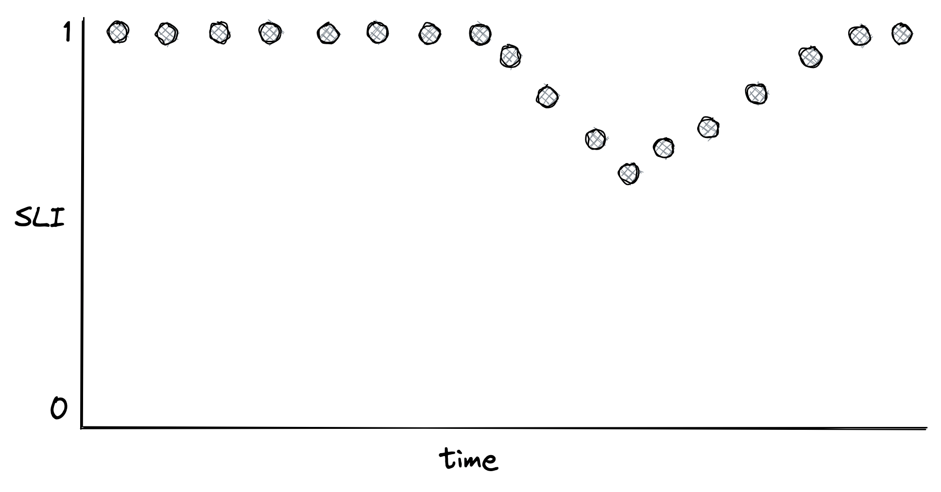
Figure 31.1: An SLI defined as the ratio of good events over the total number of events
Once we have decided what to measure, we need to decide where to measure it. Take the response time, for example. Should we measure the response time as seen by the service, load balancer, or clients? Ideally, we should select the metric that best represents the users’ experience. If that’s too costly to collect, we should pick the next best candidate. In the previous example, the client metric is the most meaningful of the lot since it accounts for delays and hiccups through the entire request path.
Now, how should we measure the response time? Measurements can be affected by many factors, such as network delays, page faults, or heavy context switching. Since every request does not take the same amount of time, response times are best represented with a distribution, which usually is right-skewed and long-tailed[8].
A distribution can be summarized with a statistic. Take the average, for example. While it has its uses, it doesn’t tell us much about the proportion of requests experiencing a specific response time, and all it takes to skew the average is one large outlier. For example, suppose we collected 100 response times, of which 99 are 1 second, and one is 10 minutes. In this case, the average is nearly 7 seconds. So even though 99% of the requests experience a response time of 1 second, the average is 7 times higher than that.
A better way to represent the distribution of response times is with percentiles. A percentile is the value below which a percentage of the response times fall. For example, if the 99th percentile is 1 second, then 99% of requests have a response time below or equal to 1 second. The upper percentiles of a response time distribution, like the 99th and 99.9th percentiles, are also called long-tail latencies. Even though only a small fraction of requests experience these extreme latencies, it can impact the most important users for the business. They are the ones that make the highest number of requests and thus have a higher chance of experiencing tail latencies. There are studies[9] that show that high latencies negatively affect revenues: a mere 100-millisecond delay in load time can hurt conversion rates by 7 percent.
Also, long-tail latencies can dramatically impact a service. For example, suppose a service on average uses about 2K threads to serve 10K requests per second. By Little’s Law[10], the average response time of a thread is 200 ms. Now, if suddenly 1% of requests start taking 20 seconds to complete (e.g., because of a congested switch and relaxed timeouts), 2K additional threads are needed to deal just with the slow requests. So the number of threads used by the service has to double to sustain the load!
Measuring long-tail latencies and keeping them in check doesn’t just make our users happy but also drastically improves the resiliency of our systems while reducing their operational costs. Intuitively, by reducing the long-tail latency (worst-case scenario), we also happen to improve the average-case scenario.
Service-level objectives
A service-level objective (SLO) defines a range of acceptable values for an SLI within which the service is considered to be in a healthy state (see Figure 31.2). An SLO sets the expectation to the service’s users of how it should behave when it’s functioning correctly. Service owners can also use SLOs to define a service-level agreement (SLA) with their users — a contractual agreement that dictates what happens when an SLO isn’t met, generally resulting in financial consequences.
For example, an SLO could define that 99% of API calls to end-point X should complete below 200 ms, as measured over a rolling window of 1 week. Another way to look at it is that it’s acceptable for up to 1% of requests within a rolling week to have a latency higher than 200 ms. That 1% is also called the error budget, which represents the number of failures that can be tolerated.
SLOs are helpful for alerting purposes and also help the team prioritize repair tasks. For example, the team could agree that when an error budget is exhausted, repair items will take precedence over new features until the SLO is repaired. Furthermore, an incident’s importance can be measured by how much of the error budget has been burned. For example, an incident that burned 20% of the error budget is more important than one that burned only 1%.
Smaller time windows force the team to act quicker and prioritize bug fixes and repair items, while longer windows are better suited to make long-term decisions about which projects to invest
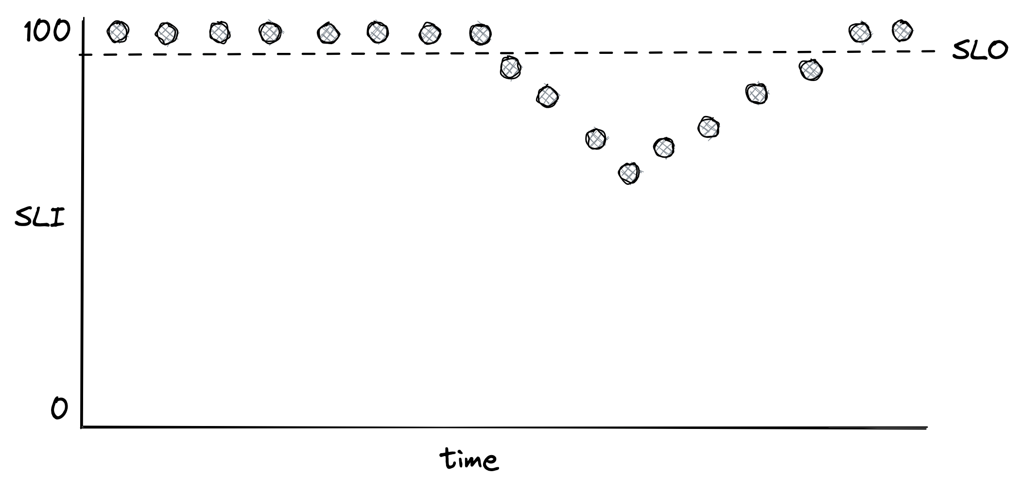
Figure 31.2: An SLO defines the range of acceptable values for an SLI.
in. Consequently, it makes sense to have multiple SLOs with different window sizes.
How strict should SLOs be? Choosing the right target range is harder than it looks. If it’s too lenient, we won’t detect user-facing issues; if it’s too strict, engineering time will be wasted with microoptimizations that yield diminishing returns. Even if we could guarantee 100% reliability for our systems (which is impossible), we can’t make guarantees for anything that our users depend on to access our service and which is outside our control, like their last-mile connection. Thus, 100% reliability doesn’t translate into a 100% reliable experience for users.
When setting the target range for SLOs, it’s reasonable to start with comfortable ranges and tighten them as we build confidence. We shouldn’t just pick targets our service meets today that might become unattainable in a year after load increases. Instead, we should work backward from what users care about. In general, anything above 3 nines of availability is very costly to achieve and provides diminishing returns.
Also, we should strive to keep things simple and have as few SLOs as possible that provide a good enough indication of the desired service level and review them periodically. For example, suppose we discover that a specific user-facing issue generated many support tickets, but none of our SLOs showed any degradation. In that case, the SLOs might be too relaxed or simply not capture a specific use case.
SLOs need to be agreed on with multiple stakeholders. If the error budget is being burned too rapidly or has been exhausted, repair items have to take priority over features. Engineers need to agree that the targets are achievable without excessive toil. Product managers also have to agree that the targets guarantee a good user experience. As Google’s SRE book mentions[11]: “if you can’t ever win a conversation about priorities by quoting a particular SLO, it’s probably not worth having that SLO.”
It’s worth mentioning that users can become over-reliant on the actual behavior of our service rather than its documented SLA. To prevent that, we can periodically inject controlled failures[12] in production — also known as chaos testing. These controlled failures ensure the dependencies can cope with the targeted service level and are not making unrealistic assumptions. As an added benefit, they also help validate that resiliency mechanisms work as expected.
Alerts
Alerting is the part of a monitoring system that triggers an action when a specific condition happens, like a metric crossing a threshold. Depending on the severity and the type of the alert, the action can range from running some automation, like restarting a service instance, to ringing the phone of a human operator who is on call. In the rest of this section, we will mostly focus on the latter case.
For an alert to be useful, it has to be actionable. The operator shouldn’t spend time exploring dashboards to assess the alert’s impact and urgency. For example, an alert signaling a spike in CPU usage is not useful as it’s not clear whether it has any impact on the system without further investigation. On the other hand, an SLO is a good candidate for an alert because it quantifies the impact on the users. The SLO’s error budget can be monitored to trigger an alert whenever a large fraction of it has been consumed.
Before discussing how to define an alert, it’s important to understand that there is a trade-off between its precision and recall. Formally, precision is the fraction of significant events (i.e., actual issues) over the total number of alerts, while recall is the ratio of significant events that triggered an alert. Alerts with low precision are noisy and often not actionable, while alerts with low recall don’t always trigger during an outage. Although it would be nice to have 100% precision and recall, improving one typically lowers the other, and so a compromise needs to be made.
Suppose we have an availability SLO of 99% over 30 days, and we would like to configure an alert for it. A naive way would be to trigger an alert whenever the availability goes below 99% within a relatively short time window, like an hour. But how much of the error budget has actually been burned by the time the alert triggers? Because the time window of the alert is one hour, and the SLO error budget is defined over 30 days, the percentage of error budget that has been spent when the alert triggers is 1 hour 30 days = 0.14%. A system is never 100% healthy, since there is always something failing at any given time. So being notified that 0.14% of the SLO’s error budget has been burned is not useful. In this case, we have a high recall but a low precision.
We can improve the alert’s precision by increasing the amount of time the condition needs to be true. The problem is that now the alert will take longer to trigger, even during an actual outage. The alternative is to alert based on how fast the error budget is burning, also known as the burn rate, which lowers the detection time. The burn rate is defined as the percentage of the error budget consumed over the percentage of the SLO time window that has elapsed — it’s the rate of exhaustion of the error budget. So using our previous example, a burn rate of 1 means the error budget will be exhausted precisely in 30 days; if the rate is 2, then it will be 15 days; if the rate is 3, it will be 10 days, and so on.
To improve recall, we can have multiple alerts with different thresholds. For example, a burn rate below 2 could be classified as a low-severity alert to be investigated during working hours, while a burn rate over 10 could trigger an automated call to an engineer. The SRE workbook has some great examples[13] of how to configure alerts based on burn rates.
While the majority of alerts should be based on SLOs, some should trigger for known failure modes that we haven’t had the time to design or debug away. For example, suppose we know a service suffers from a memory leak that has led to an incident in the past, but we haven’t yet managed to track down the root cause. In this case, as a temporary mitigation, we could define an alert that triggers an automated restart when a service instance is running out of memory.
Dashboards
After alerting, the other main use case for metrics is to power real-time dashboards that display the overall health of a system. Unfortunately, dashboards can easily become a dumping ground for charts that end up being forgotten, have questionable usefulness, or are just plain confusing. Good dashboards don’t happen by coincidence. In this section, we will discuss some of the best practices for creating useful dashboards.
When creating a dashboard, the first decision we have to make is to decide who the audience is[14] and what they are looking for. Then, given the audience, we can work backward to decide which charts, and therefore metrics, to include.
The categories of dashboards presented here (see Figure 31.3) are by no means standard but should give you an idea of how to organize dashboards.
SLO dashboard
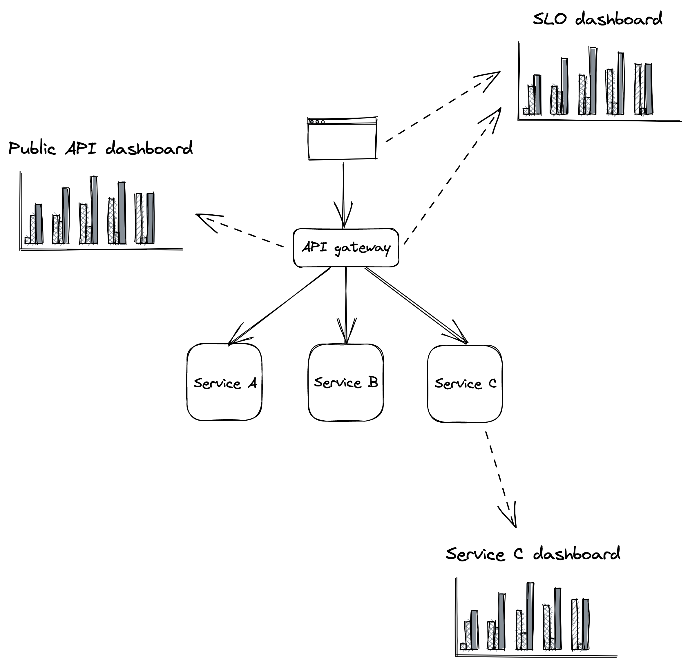
Figure 31.3: Dashboards should be tailored to their audience.
The SLO summary dashboard is designed to be used by various stakeholders from across the organization to gain visibility into the system’s health as represented by its SLOs. During an incident, this dashboard quantifies the impact the incident is having on the users.
Public API dashboard
This dashboard displays metrics about the system’s public API endpoints, which helps operators identify problematic paths during an incident. For each endpoint, the dashboard exposes several metrics related to request messages, request handling, and response messages, like:
- Number of requests received or messages pulled from a mes-
saging broker, request size statistics, authentication issues, etc. • Request handling duration, availability and response time of external dependencies, etc. • Counts per response type, size of responses, etc.
Service dashboard
A service dashboard displays service-specific implementation details, which require an in-depth understanding of its inner workings. Unlike the previous dashboards, this one is primarily used by the team that owns the service. Beyond service-specific metrics, a service dashboard should also contain metrics of upstream dependencies like load balancers and messaging queues and downstream dependencies like data stores.
This dashboard offers a first entry point into what’s going on within the service when debugging. As we will later learn when discussing observability, this high-level view is just the starting point. The operator typically drills down into the metrics by segmenting them further and eventually reaches for raw logs and traces to get more detail.
Best practices
As new metrics are added and old ones removed, charts and dashboards need to be modified and kept in sync across multiple environments (e.g., pre-production and production). The most effective way to achieve that is by defining dashboards and charts with a domain-specific language and version-controlling them just like code. This allows dashboards to be updated from the same pull request that contains related code changes without manually updating dashboards, which is error-prone.
As dashboards render top to bottom, the most important charts should always be located at the very top. Also, charts should be rendered with a default timezone, like UTC, to ease the communication between people located in different parts of the world when looking at the same data.
All charts in the same dashboard should use the same time resolution (e.g., 1 minute, 5 minutes, 1 hour, etc.) and range (24 hours, 7 days, etc.). This makes it easy to visually correlate anomalies across charts in the same dashboard. We can pick the default time range and resolution based on the dashboard’s most common use case. For example, a 1-hour range with a 1-minute resolution is best for monitoring an ongoing incident, while a 1-year range with a 1-day resolution is best for capacity planning.
We should keep the number of data points and metrics on the same chart to a minimum. Rendering too many points doesn’t just make charts slow to download/render but also makes it hard to interpret them and spot anomalies.
A chart should contain only metrics with similar ranges (min and max values); otherwise, the metric with the largest range can completely hide the others with smaller ranges. For that reason, it makes sense to split related statistics for the same metric into multiple charts. For example, the 10th percentile, average and 90th percentile of a metric can be displayed in one chart, and the 0.1th percentile, 99.9th percentile, minimum and maximum in another.
A chart should also contain useful annotations, like:
- a description of the chart with links to runbooks, related dashboards, and escalation contacts;
- a horizontal line for each configured alert threshold, if any;
- a vertical line for each relevant deployment.
Metrics that are only emitted when an error condition occurs can be hard to interpret as charts will show wide gaps between the data points, leaving the operator wondering whether the service stopped emitting that metric due to a bug. To avoid this, it’s best practice to emit a metric using a value of zero in the absence of an error and a value of 1 in the presence of it.
Being on call
A healthy on-call rotation is only possible when services are built from the ground up with reliability and operability in mind. By making the developers responsible for operating what they build, they are incentivized to reduce the operational toll to a minimum. They are also in the best position to be on call since they are intimately familiar with the system’s architecture, brick walls, and trade-offs.
Being on call can be very stressful. Even when there are no callouts, just the thought of not having the usual freedom outside of regular working hours can cause a great deal of anxiety. This is why being on call should be compensated, and there shouldn’t be any expectations for the on-call engineer to make any progress on feature work. Since they will be interrupted by alerts, they should make the most of it and be given free rein to improve the on-call experience by, e.g., revising dashboards or improving resiliency mechanisms.
Achieving a healthy on-call rotation is only possible when alerts are actionable. When an alert triggers, to the very least, it should link to relevant dashboards and a run-book that lists the actions the engineer should take[15]. Unless the alert was a false positive, all actions taken by the operator should be communicated into a shared channel like a global chat accessible by other teams. This allows other engineers to chime in, track the incident’s progress, and more easily hand over an ongoing incident to someone else.
The first step to address an alert is to mitigate it, not fix the underlying root cause that created it. A new artifact has been rolled out that degrades the service? Roll it back. The service can’t cope with the load even though it hasn’t increased? Scale it out.
Once the incident has been mitigated, the next step is to understand the root cause and come up with ways to prevent it from happening again. The greater the impact was, as measured by the SLOs, the more time we should spend on this. Incidents that burned a significant fraction of an SLO’s error budget require a formal postmortem. The goal of the postmortem is to understand the incident’s root cause and come up with a set of repair items that will prevent it from happening again. Ideally, there should also be an agreement in the team that if an SLO’s error budget is burned or the number of alerts spirals out of control, the whole team stops working on new features to focus exclusively on reliability until a healthy on-call rotation has been restored.
The SRE books[16] provide a wealth of information and best practices regarding setting up a healthy on-call rotation.
Observability
Video coming soon. Start with the reading below.
A distributed system is never 100% healthy since, at any given time, there is always something failing. A whole range of failure modes can be tolerated, thanks to relaxed consistency models and resiliency mechanisms like rate limiting, retries, and circuit breakers. But, unfortunately, they also increase the system’s complexity. And with more complexity, it becomes increasingly harder to reason about the multitude of emergent behaviors the system might experience, which are impossible to predict up front.
As discussed earlier, human operators are still a fundamental part of operating a service as there are things that can’t be automated, like debugging the root cause of a failure. When debugging, the operator makes a hypothesis and tries to validate it. For example, the operator might get suspicious after noticing that the variance of their service’s response time has increased slowly but steadily over the past weeks, indicating that some requests take much longer than others. After correlating the increase in variance with an increase in traffic, the operator hypothesizes that the service is getting closer to hitting a constraint, like a resource limit. But metrics and charts alone won’t help to validate this hypothesis.
Observability is a set of tools that provide granular insights into a system in production, allowing one to understand its emergent behaviors. A good observability platform strives to minimize the time it takes to validate hypotheses. This requires granular events with rich contexts since it’s impossible to know up front what will be useful in the future.
At the core of observability, we find telemetry sources like metrics, event logs, and traces. Metrics are stored in time-series data stores that have high throughput but struggle with high dimensionality. Conversely, event logs and traces end up in stores that can handle high-dimensional data[1] but struggle with high throughput. Metrics are mainly used for monitoring, while event logs and traces are mainly for debugging.
Observability is a superset of monitoring. While monitoring is focused exclusively on tracking a system’s health, observability also provides tools to understand and debug the system. For example, monitoring on its own is good at detecting failure symptoms but less so at explaining their root cause (see Figure 32.1).
Logs
A log is an immutable list of time-stamped events that happened over time. An event can have different formats. In its simplest form, it’s just free-form text. It can also be structured and represented with a textual format like JSON or a binary one like Protobuf. When structured, an event is typically represented with a bag of key-value pairs:
{
  "failureCount": 1,
  "serviceRegion": "EastUs2",
  "timestamp": 1614438079
}
Logs can originate from our services or external dependencies, like
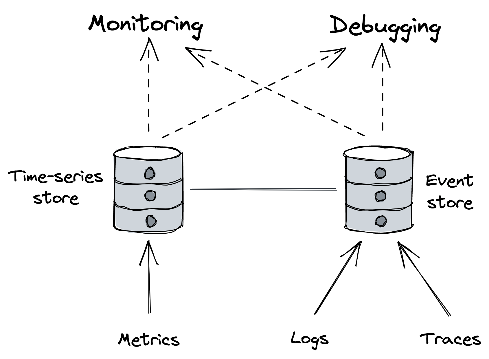
Figure 32.1: Observability is a superset of monitoring.
message brokers, proxies, data stores, etc. Most languages offer libraries that make it easy to emit structured logs. Logs are typically dumped to disk files, which are sent by an agent to an external log collector asynchronously, like an ELK stack[2] or AWS CloudWatch logs.
Logs provide a wealth of information about everything that’s happening in a service, assuming it was instrumented properly. They are particularly helpful for debugging purposes, as they allow us to trace back the root cause from a symptom, like a service instance crash. They also help investigate long-tail behaviors that are invisible to metrics summarized with averages and percentiles, which can’t explain why a specific user request is failing.
Logs are simple to emit, particularly so free-form textual ones. But that’s pretty much the only advantage they have compared to metrics and other telemetry data. Logging libraries can add overhead to our services if misused, especially when they are not asynchronous and block while writing to disk. Also, if the disk fills up due to excessive logging, at best we lose logs, and at worst, the service instance stops working correctly.
Ingesting, processing, and storing massive troves of data is not cheap either, no matter whether we plan to do this in-house or use a third-party service. Although structured binary logs are more efficient than textual ones, they are still expensive due to their high dimensionality.
Finally, but no less importantly, logs have a low signal-to-noise ratio because they are fine-grained and service-specific, making it challenging to extract useful information.
Best practices
To make the job of the engineer drilling into the logs less painful, all the data about a specific work unit should be stored in a single event. A work unit typically corresponds to a request or a message pulled from a queue. To effectively implement this pattern, code paths handling work units need to pass around a context object containing the event being built.
An event should contain useful information about the work unit, like who created it, what it was for, and whether it succeeded or failed. It should also include measurements, like how long specific operations took. In addition, every network call performed within the work unit needs to be instrumented and log, e.g., its response time and status code. Finally, data logged to the event should be sanitized and stripped of potentially sensitive properties that developers shouldn’t have access to, like users’ personal data.
Collating all data within a single event for a work unit minimizes the need for joins but doesn’t completely eliminate it. For example, if a service calls another downstream, we will have to perform a join to correlate the caller’s event log with the callee’s one to understand why the remote call failed. To make that possible, every event should include the identifier of the request (or message) for the work unit.
Costs
There are various ways to keep the costs of logging under control. A simple approach is to have different logging levels (e.g., debug, info, warning, error) controlled by a dynamic knob that determines which ones are emitted. This allows operators to increase the logging verbosity for investigation purposes and reduce costs when granular logs aren’t needed.
Sampling[3] is another tool at our disposal for reducing verbosity. For example, a service could log only every nth event. Additionally, events can also be prioritized based on their expected signalto-noise ratio: logging failed requests should have a higher sampling frequency than logging successful ones.
The options discussed so far only reduce the logging verbosity on a single node. As we scale out and add more nodes, the logging volume will necessarily increase. Even with the best intentions, someone could check in a bug that leads to excessive logging. To avoid costs soaring through the roof or overloading our log collector service, log collectors need to be able to rate-limit requests.
Of course, we can always decide to create in-memory aggregates (e.g., metrics) from the measurements collected in events and emit just those rather than raw logs. However, by doing so, we trade off the ability to drill down into the aggregates if needed.
Traces
Tracing captures the entire lifespan of a request as it propagates throughout the services of a distributed system. A trace is a list of causally-related spans that represent the execution flow of a request in a system. A span represents an interval of time that maps to a logical operation or work unit and contains a bag of key-value pairs (see Figure 32.2).
When a request begins, it’s assigned a unique trace ID. The trace ID is propagated from one stage to another at every fork in the local execution flow from one thread to another, and from caller to callee in a network call (through HTTP headers, for example).
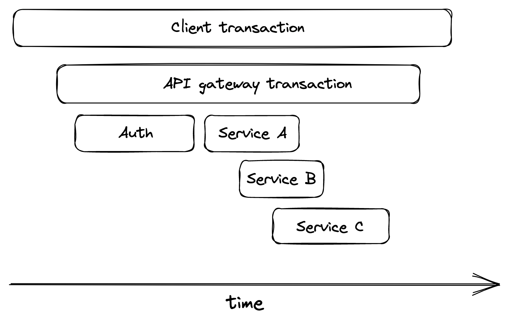
Figure 32.2: An execution flow can be represented with spans.
Each stage is represented with a span — an event containing the trace ID.
When a span ends, it’s emitted to a collector service, which assembles it into a trace by stitching it together with the other spans belonging to the same trace. Popular distributed tracing collectors include Open Zipkin[4] and AWS X-ray[5].
Traces allow developers to:
- debug issues affecting very specific requests, which can be used to investigate failed requests raised by customers in support tickets;
- debug rare issues that affect only an extremely small fraction of requests;
- debug issues that affect a large fraction of requests that have something in common, like high response times for requests that hit a specific subset of service instances;
- identify bottlenecks in the end-to-end request path;
- identify which users hit which downstream services and
in what proportion (also referred to as resource attribution), which can be used for rate-limiting or billing purposes.
Tracing is challenging to retrofit into an existing system since it requires every component in the request path to be modified to propagate the trace context from one stage to the other. And it’s not just the components that are under our control that need to support tracing; third-party frameworks, libraries, and services need to as well.[6].
Putting it all together
The main drawback of event logs is that they are fine-grained and service-specific. When a user request flows through a system, it can pass through several services. A specific event only contains information for the work unit of one specific service, so it can’t be of much use for debugging the entire request flow. Similarly, a single event doesn’t give much information about the health or state of a specific service.
This is where metrics and traces come in. We can think of them as abstractions, or derived views, built from event logs and optimized for specific use cases. A metric is a time series of summary statistics derived by aggregating counters or observations over multiple events. For example, we could emit counters in events and have the backend roll them up into metrics as they are ingested. In fact, this is how some metric-collection systems work.
Similarly, a trace can be derived by aggregating all events belonging to the lifecycle of a specific user request into an ordered list. Just like in the previous case, we can emit individual span events and have the backend aggregate them together into traces.
Manageability
Video coming soon. Start with the reading below.
Operators use observability tools to understand the behavior of their application, but they also need a way to modify the behavior without code changes. One example of this is releasing a new version of an application to production, which we discussed earlier. Another example is changing the way an application behaves by modifying its configuration.
An application generally depends on a variety of configuration settings. Some affect its behavior, like the maximum size of an internal cache, while others contain secrets, like credentials to access external data stores. Because settings vary by environment and can contain sensitive information, they should not be hardcoded.
To decouple the application from its configuration, the configuration can be persisted in a dedicated store[1] like AWS AppConfig[2] or Azure App Configuration[3].
At deployment time, the CD pipeline can read the configuration from the store and pass it to the application through environment variables. The drawback of this approach is that the configuration cannot be changed without redeploying the application.
For the application to be able to react to configuration changes, it needs to periodically re-read the configuration during run time and apply the changes. For example, if the constructor of an HTTP handler depends on a specific configuration setting, the handler needs to be re-created when that setting changes.
Once it’s possible to change configuration settings dynamically, new features can be released with settings to toggle (enable/disable) them. This allows a build to be released with a new feature disabled at first. Later, the feature can be enabled for a fraction of application instances (or users) to build up confidence that it’s working as intended before it’s fully rolled out. Similarly, the same mechanism can be used to perform A/B tests[4].
If you have spent even a few months in a team that operates a production service, you should be very familiar with the topics discussed in this part. Although we would all love to design new large-scale systems and move on, the reality is that the majority of the time is spent in maintenance activities, such as fixing bugs, adding new features to existing services, and operating production services.
In my opinion, the only way to become a better system designer is to embrace these maintenance activities and aspire to make your systems easy to modify, extend and operate so that they are easy to maintain. By doing so, you will pick up a “sixth sense” that will allow you to critique the design of third-party systems and ultimately make you a better systems designer/builder.
So my advice to you is to use every chance you get to learn from production services. Be on call for your services. Participate in as many post-mortems as you can and relentlessly ask yourself how an incident could have been avoided. These activities will pay off in the long term a lot more than reading about the latest architectural patterns and trends.
Final words
Video coming soon. Start with the reading below.
Congratulations, you reached the end of this learning path! I hope you learned something you didn’t know before and perhaps even had a few “aha” moments. Although this is the end of this learning path, it’s just the beginning of your journey.
The best way to continue your learning journey is to go out in the world and design, build and maintain large-scale systems. Some of the best-paid jobs in the industry involve building such systems, and there is no shortage of demand. The second-best way is by reading industry papers, which provide a wealth of knowledge about distributed systems that have stood the test of time. And after reading this module, these papers should be accessible to you.
For example, you could start with “Windows Azure Storage: A Highly Available Cloud Storage Service with Strong Consistency”[1], which describes Azure’s cloud storage system. Azure’s cloud storage is the core building block on top of which Microsoft built many other successful products. One of the key design decisions was to guarantee strong consistency, making the application developers’ job much easier. I like this paper a lot because it touches upon many of the concepts discussed in this module.
Once you have digested the Azure storage paper, I suggest reading “Azure Data Explorer: a big data analytics cloud platform optimized for interactive, ad-hoc queries over structured, semi-structured and unstructured data”[2]. This paper discusses the implementation of a cloud-native event store built on top of Azure’s cloud storage — a great example of how these large-scale systems compose on top of each other.
If any concept is new to you or unclear, follow your curiosity down the rabbit hole by exploring referenced papers.[3]. As a bonus exercise, this module is sprinkled with great papers and references. Read them all to complete all the side quests!
In terms of book recommendations, Martin Kleppman’s “Designing Data-Intensive Applications”4 is a must-read. The book describes the pros and cons of various technologies for processing and storing data. Also, for some more high-level case studies, check out Alex Xu’s “System Design Interview”5 — it’s a good read even if you aren’t preparing for interviews.
As no book is ever perfect, I’m always happy to receive feedback. So if you have found an error, have an idea for improvement, or simply want to comment on something, always feel free to write me6. I love connecting with readers.
Finally, please consider leaving a review on Goodreads or Amazon if you liked this learning path. It makes all the difference to prospective readers.
Module references
References
- Cindy Sridharan wrote a great blog post series on the topic, see “Testing Microservices, the sane way,” https://copyconstruct.medium.com/testing-microservices-the-sane-way-9bb31d158c16
- The kind of unit test I have in mind is the sociable kind; see “On the Diverse And Fantastical Shapes of Testing,” https://martinfowler.com/articles/2021-test-shapes.html
- “IntegrationTest,” https://martinfowler.com/bliki/IntegrationTest.html
- “Software Engineering at Google: Lessons Learned from Programming Over Time,” https://www.amazon.com/dp/B0859PF5HB
- “ContractTest,” https://martinfowler.com/bliki/ContractTest.html
- “The TLA+ Home Page,” https://lamport.azurewebsites.net/tla/tla.html
- TLA stands for Temporal Logic of Actions.
- “Industrial Use of TLA+,” https://lamport.azurewebsites.net/tla/industrial-use.html
References
- There could be multiple breaking changes, actually.
- “What is Infrastructure as Code?,” https://docs.microsoft.com/en-us/devops/deliver/what-is-infrastructure-as-code
- “Terraform: an open-source infrastructure as code software tool,” https://www.terraform.io/
- “Automating safe, hands-off deployments,” https://aws.amazon.com/builders-library/automating-safe-hands-off-deployments/
- This is also referred to as canary testing.
- CD pipelines can be configured to run only during business hours to minimize the disruption to on-call engineers.
- “Ensuring rollback safety during deployments,” https://aws.amazon.com/builders-library/ensuring-rollback-safety-during-deployments/
References
- “Measure Anything, Measure Everything,” https://codeascraft.com/2011/02/15/measure-anything-measure-everything/
- “Using synthetic monitoring,” https://docs.aws.amazon.com/AmazonCloudWatch/latest/monitoring/CloudWatch_Synthetics_Canaries.html
- I have omitted error handling for simplicity.
- We will talk more about event logs in Logs in Observability; for now, assume an event is just a dictionary.
- “Log-based metrics in Application Insights,” https://docs.microsoft.com/en-us/azure/azure-monitor/app/pre-aggregated-metrics-log-metrics#log-based-metrics
- “Amazon CloudWatch concepts,” https://docs.aws.amazon.com/AmazonCloudWatch/latest/monitoring/cloudwatch_concepts.html
- like, e.g., Druid; see “A Real-time Analytical Data Store,” http://static.druid.io/docs/druid.pdf
- “latency: a primer,” https://igor.io/latency/
- “Akamai Online Retail Performance Report: Milliseconds Are Critical,” https://www.akamai.com/newsroom/press-release/akamai-releases-spring-2017-state-of-online-retail-performance-report
- Little’s law says the average number of items in a system equals the average rate at which new items arrive multiplied by the average time an item spends in the system; see “Back of the envelope estimation hacks,” https://robertovitillo.com/back-of-the-envelope-estimation-hacks/
- “Service Level Objectives,” https://sre.google/sre-book/service-level-objectives/
- “Chaos engineering,” https://en.wikipedia.org/wiki/Chaos_engineering
- “Alerting on SLOs,” https://sre.google/workbook/alerting-on-slos/
- “Building dashboards for operational visibility,” https://aws.amazon.com/builders-library/building-dashboards-for-operational-visibility
- Ideally, we should automate what we can to minimize manual actions that operators need to perform. As it turns out, machines are good at following instructions.
- “SRE Books,” https://sre.google/books/
References
- Azure Data Explorer is one such event store, see “Azure Data Explorer: a big data analytics cloud platform optimized for interactive, adhoc queries over structured, semi-structured and unstructured data,” https://azure.microsoft.com/mediahandler/files/resourcefiles/azure-data-explorer/Azure_Data_Explorer_white_paper.pdf
- “What is the ELK Stack?,” https://www.elastic.co/what-is/elk-stack
- “Dynamic Sampling by Example,” https://www.honeycomb.io/blog/dynamic-sampling-by-example/
- “Zipkin: a distributed tracing system,” https://zipkin.io/
- “AWS X-Ray,” https://aws.amazon.com/xray/
- The service mesh pattern can help retrofit tracing.
References
- “Continuous Configuration at the Speed of Sound,” https://www.allthingsdistributed.com/2021/08/continuous-configuration-on-aws.html
- “AWS AppConfig Documentation,” https://docs.aws.amazon.com/appconfig/
- “Azure App Configuration,” https://azure.microsoft.com/en-us/services/app-configuration/
- “A/B testing,” https://en.wikipedia.org/wiki/A/B_testing
References
- “Windows Azure Storage: A Highly Available Cloud Storage Service with Strong Consistency,” https://sigops.org/s/conferences/sosp/2011/current/2011-Cascais/printable/11-calder.pdf
- “Azure Data Explorer: a big data analytics cloud platform optimized for interactive, ad-hoc queries over structured, semi-structured and unstructured data,” https://azure.microsoft.com/mediahandler/files/resourcefiles/azure-data-explorer/Azure_Data_Explorer_white_paper.pdf
- If you are new to reading papers, use the three-pass approach by S. Keshav, see “How to Read a Paper,” https://web.stanford.edu/class/ee384m/Handouts/HowtoReadPaper.pdf