Study one concept at a time. Open the guided module →
Coordination
Overview: Coordination
Video coming soon. Start with the reading below.
“Here is a Raft joke. It is really a Paxos joke, but easier to follow.”
– Aleksey Charapko
So far, we have learned how to get processes to communicate reliably and securely with each other. We didn’t go into all this trouble just for the sake of it, though. Our ultimate goal is to build a distributed application made of a group of processes that gives its users the illusion they are interacting with one coherent node. Although achieving a perfect illusion is not always possible or desirable, some degree of coordination is always needed to build a distributed application.
In this part, we will explore the core distributed algorithms at the heart of distributed applications. This is the most challenging part of this learning path since it contains the most theory, but also the most rewarding one once you understand it. If something isn’t clear during your first read, try to read it again and engage with the content by following the references in the text. Some of these references point to papers, but don’t be intimidated. You will find that many papers are a lot easier to digest and more practical than you think. There is only so much depth a book can go into, and if you want to become an expert, reading papers should become a habit.
System models (lesson 03.02) introduces formal models that categorize systems based on what guarantees they offer about the behavior of processes, communication links, and timing; they allow us to reason about distributed systems by abstracting away the implementation details.
Failure detection (lesson 03.03) describes how to detect that a remote process is unreachable. Failure detection is a crucial component of any distributed system. Because networks are unreliable, and processes can crash at any time, without failure detection a process trying to communicate with another could hang forever.
Time (lesson 03.04) dives into the concept of time and order. We will first learn why agreeing on the time an event happened in a distributed system is much harder than it looks and then discuss a solution based on clocks that don’t measure the passing of time.
Leader election (lesson 03.05) describes how a group of processes can elect a leader that can perform privileged operations, like accessing a shared resource or coordinating the actions of other processes.
Replication (lesson 03.06) introduces one of the fundamental challenges in distributed systems: replicating data across multiple processes. This lesson also discusses the implications of the CAP and PACELC theorems, namely the tradeoff between consistency and availability/performance.
Coordination avoidance (lesson 03.07) explores weaker consistency models for replicated data, like strong eventual consistency and causal consistency, which allow us to build consistent, available, and partition-tolerant systems.
Transactions (lesson 03.08) dives into the implementation of ACID transactions that span data partitioned among multiple processes or services. Transactions relieve us from a whole range of possible failure scenarios so that we can focus on the actual application logic rather than all the possible things that can go wrong.
Asynchronous transactions (lesson 03.09) discusses how to implement long-running atomic transactions that don’t block by sacrificing the isolation guarantees of ACID. This lesson is particularly relevant in practice since it showcases techniques commonly used in microservice architectures.
System models
Video coming soon. Start with the reading below.
To reason about distributed systems, we need to define precisely what can and can’t happen. A system model encodes expectations about the behavior of processes, communication links, and timing; think of it as a set of assumptions that allow us to reason about distributed systems by ignoring the complexity of the actual technologies used to implement them.
For example, these are some common models for communication links:
- The fair-loss link model assumes that messages may be lost and duplicated, but if the sender keeps retransmitting a message, eventually it will be delivered to the destination.
- The reliable link model assumes that a message is delivered exactly once, without loss or duplication. A reliable link can be implemented on top of a fair-loss one by de-duplicating messages at the receiving side.
- The authenticated reliable link model makes the same assumptions as the reliable link but additionally assumes that the receiver can authenticate the sender.
Even though these models are just abstractions of real communication links, they are useful to verify the correctness of algorithms. And, as we have seen in the earlier lessons, it’s possible to build a reliable and authenticated communication link on top of a fair-loss one. For example, TCP implements reliable transmission (and more), while TLS implements authentication (and more).
Similarly, we can model the behavior of processes based on the type of failures we expect to happen:
- The arbitrary-fault model assumes that a process can deviate from its algorithm in arbitrary ways, leading to crashes or unexpected behaviors caused by bugs or malicious activity. For historical reasons, this model is also referred to as the “Byzantine” model. More interestingly, it can be theoretically
proven that a system using this model can tolerate up to [1]
3 of faulty processes[1] and still operate correctly. • The crash-recovery model assumes that a process doesn’t deviate from its algorithm but can crash and restart at any time, losing its in-memory state. • The crash-stop model assumes that a process doesn’t deviate from its algorithm but doesn’t come back online if it crashes. Although this seems unrealistic for software crashes, it models unrecoverable hardware faults and generally makes the algorithms simpler.
The arbitrary-fault model is typically used to model safety-critical systems like airplane engines, nuclear power plants, and systems where a single entity doesn’t fully control all the processes (e.g., digital cryptocurrencies such as Bitcoin). These use cases are outside this learning path’s scope, and the algorithms presented here will generally assume a crash-recovery model.
Finally, we can also model timing assumptions:
- The synchronous model assumes that sending a message or executing an operation never takes more than a certain amount of time. This is not very realistic for the type of systems we care about, where we know that sending messages over the network can potentially take a very long
time, and processes can be slowed down by, e.g., garbage collection cycles or page faults. • The asynchronous model assumes that sending a message or executing an operation on a process can take an unbounded amount of time. Unfortunately, many problems can’t be solved under this assumption; if sending messages can take an infinite amount of time, algorithms can get stuck and not make any progress at all. Nevertheless, this model is useful because it’s simpler than models that make timing assumptions, and therefore algorithms based on it are also easier to implement[2]. • The partially synchronous model assumes that the system behaves synchronously most of the time. This model is typically representative enough of real-world systems.
In the rest of this learning path, we will generally assume a system model with fair-loss links, crash-recovery processes, and partial synchrony. If you are curious and want to learn more about other system models, “Introduction to Reliable and Secure Distributed Programming”[3] is an excellent theoretical book that explores distributed algorithms for a variety of models not considered in this text.
But remember, models are just an abstraction of reality[4] since they don’t represent the real world with all its nuances. So, as you read along, question the models’ assumptions and try to imagine how algorithms that rely on them could break in practice.
Failure detection
Video coming soon. Start with the reading below.
Several things can go wrong when a client sends a request to a server. In the best case, the client sends a request and receives a response. But what if no response comes back after some time? In that case, it’s impossible to tell whether the server is just very slow, it crashed, or a message couldn’t be delivered because of a network issue (see Figure 7.1).
In the worst case, the client will wait forever for a response that will never arrive. The best it can do is make an educated guess, after some time has passed, on whether the server is unavailable. The client can configure a timeout to trigger if it hasn’t received a response from the server after a certain amount of time. If and when the timeout triggers, the client considers the server unavailable and either throws an error or retries the request.
The tricky part is deciding how long to wait for the timeout to trigger. If the delay is too short, the client might wrongly assume the server is unavailable; if the delay is too long, the client might waste time waiting for a response that will never arrive. In summary, it’s not possible to build a perfect failure detector.
But a process doesn’t need to wait to send a message to find out that the destination is not reachable. It can also proactively try to maintain a list of available processes using pings or heartbeats.
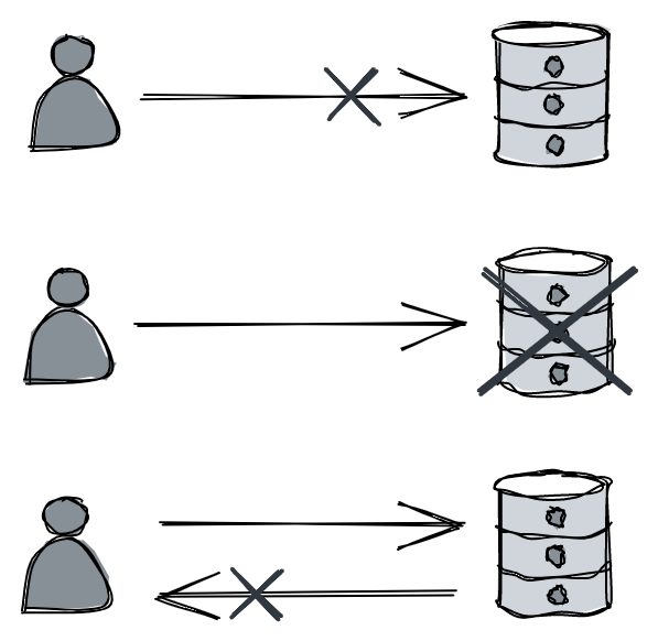
Figure 7.1: The client can’t tell whether the server is slow, it crashed or a message was delayed/dropped because of a network issue.
A ping is a periodic request that a process sends to another to check whether it’s still available. The process expects a response to the ping within a specific time frame. If no response is received, a time-out triggers and the destination is considered unavailable. However, the process will continue to send pings to it to detect if and when it comes back online.
A heartbeat is a message that a process periodically sends to another. If the destination doesn’t receive a heartbeat within a specific time frame, it triggers a timeout and considers the process unavailable. But if the process comes back to life later and starts sending out heartbeats, it will eventually be considered to be available again.
Pings and heartbeats are generally used for processes that interact with each other frequently, in situations where an action needs to be taken as soon as one of them is no longer reachable. In other circumstances, detecting failures just at communication time is good enough.
Time
Video coming soon. Start with the reading below.
Time is an essential concept in any software application; even more so in distributed ones. We have seen it play a crucial role in the network stack (e.g., DNS record TTL) and failure detection (timeouts). Another important use of it is for ordering events.
The flow of execution of a single-threaded application is simple to understand because every operation executes sequentially in time, one after the other. But in a distributed system, there is no shared global clock that all processes agree on that can be used to order operations. And, to make matters worse, processes can run concurrently.
It’s challenging to build distributed applications that work as intended without knowing whether one operation happened before another. In this lesson, we will learn about a family of clocks that can be used to work out the order of operations across processes in a distributed system.
Physical clocks
A process has access to a physical wall-time clock. The most common type is based on a vibrating quartz crystal, which is cheap but not very accurate. Depending on manufacturing differences and external temperature, one quartz clock can run slightly faster or slower than others. The rate at which a clock runs faster or slower is also called clock drift. In contrast, the difference between two clocks at a specific point in time is referred to as clock skew.
Because quartz clocks drift, they need to be synced periodically with machines that have access to higher-accuracy clocks, like atomic ones. Atomic clocks[1] measure time based on quantummechanical properties of atoms. They are significantly more expensive than quartz clocks and accurate to 1 second in 3 million years.
The synchronization between clocks can be implemented with a protocol, and the challenge is to do so despite the unpredictable latencies introduced by the network. The most commonly used protocol is the Network Time Protocol (NTP[2]). In NTP, a client estimates the clock skew by receiving a timestamp from a NTP server and correcting it with the estimated network latency. With an estimate of the clock skew, the client can adjust its clock. However, this causes the clock to jump forward or backward in time, which creates a problem when comparing timestamps. For example, an operation that runs after another could have an earlier timestamp because the clock jumped back in time between the two operations.
Luckily, most operating systems offer a different type of clock that is not affected by time jumps: a monotonic clock. A monotonic clock measures the number of seconds elapsed since an arbitrary point in time (e.g., boot time) and can only move forward. A monotonic clock is useful for measuring how much time has elapsed between two timestamps on the same node. However, monotonic clocks are of no use for comparing timestamps of different nodes.
Since we don’t have a way to synchronize wall-time clocks across processes perfectly, we can’t depend on them for ordering operations across nodes. To solve this problem, we need to look at it from another angle. We know that two operations can’t run concurrently in a single-threaded process as one must happen before the other. This happened-before relationship creates a causal bond between the two operations, since the one that happens first can have side-effects that affect the operation that comes after it. We can use this intuition to build a different type of clock that isn’t tied to the physical concept of time but rather captures the causal relationship between operations: a logical clock.
Logical clocks
A logical clock measures the passing of time in terms of logical operations, not wall-clock time. The simplest possible logical clock is a counter, incremented before an operation is executed. Doing so ensures that each operation has a distinct logical timestamp. If two operations execute on the same process, then necessarily one must come before the other, and their logical timestamps will reflect that. But what about operations executed on different processes?
Imagine sending an email to a friend. Any actions you did before sending that email, like drinking coffee, must have happened before the actions your friend took after receiving the email. Similarly, when one process sends a message to another, a so-called synchronization point is created. The operations executed by the sender before the message was sent must have happened before the operations that the receiver executed after receiving it.
A Lamport clock[3] is a logical clock based on this idea. To implement it, each process in the system needs to have a local counter that follows specific rules:
- The counter is initialized with 0.
- The process increments its counter by 1 before executing an operation.
- When the process sends a message, it increments its counter by 1 and sends a copy of it in the message.
- When the process receives a message, it merges the counter
it received with its local counter by taking the maximum of the two. Finally, it increments the counter by 1.
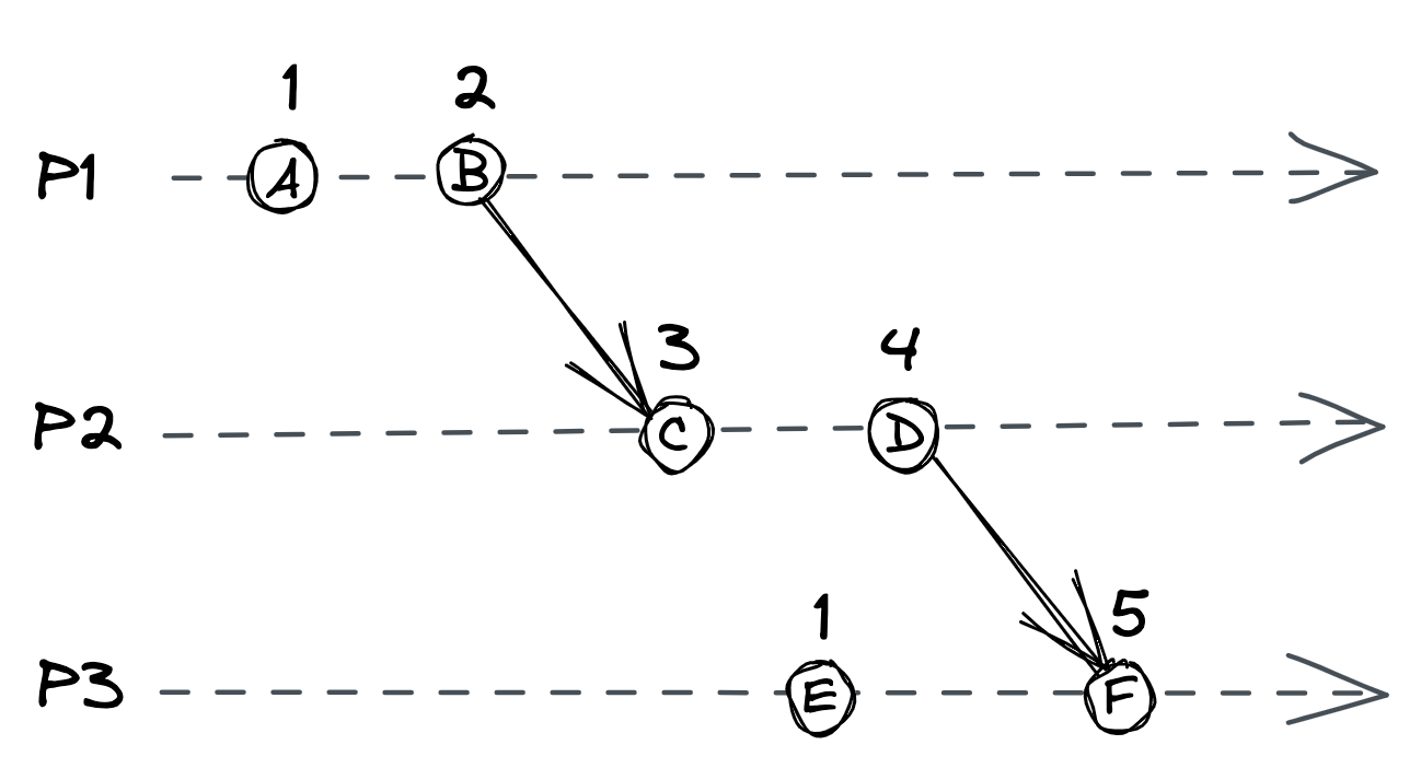
Figure 8.1: Three processes using Lamport clocks. For example, because D happened before F, D’s logical timestamp is less than F’s.
Although the Lamport clock assumes a crash-stop model, a crashrecovery one can be supported by e.g., persisting the clock’s state on disk.
The rules guarantee that if operation O1 happened-before operation O2, the logical timestamp of O1 is less than the one of O2. In the example shown in Figure 8.1, operation D happened-before F, and their logical timestamps, 4 and 5, reflect that.
However, two unrelated operations can have the same logical timestamp. For example, the logical timestamps of operations A and E are equal to 1. To create a strict total order, we can arbitrarily order the processes to break ties. For example, if we used the process IDs in Figure 8.1 to break ties (1, 2, and 3), E’s timestamp would be greater than A’s.
Regardless of whether ties are broken, the order of logical timestamps doesn’t imply a causal relationship. For example, in Figure 8.1, operation E didn’t happen-before C, even if their timestamps appear to imply it. To guarantee this relationship, we have to use a different type of logical clock: a vector clock.
Vector clocks
A vector clock[4] is a logical clock that guarantees that if a logical timestamp is less than another, then the former must have happened-before the latter. A vector clock is implemented with an array of counters, one for each process in the system. And, as with Lamport clocks, each process has its local copy.
For example, suppose the system is composed of three processes, P1, P2, and P3. In this case, each process has a local vector clock implemented with an array[5] of three counters [CP1, CP2, CP3]. The first counter in the array is associated with P1, the second with P2, and the third with P3.
A process updates its local vector clock based on the following rules:
- Initially, the counters in the array are set to 0.
- When an operation occurs, the process increments its counter in the array by 1.
- When the process sends a message, it increments its counter in the array by 1 and sends a copy of the array with the message.
- When the process receives a message, it merges the array it received with the local one by taking the maximum of the two arrays element-wise. Finally, it increments its counter in the array by 1.
The beauty of vector clock timestamps is that they can be partially ordered[6]; given two operations O1 and O2 with timestamps T1 and T2, if:
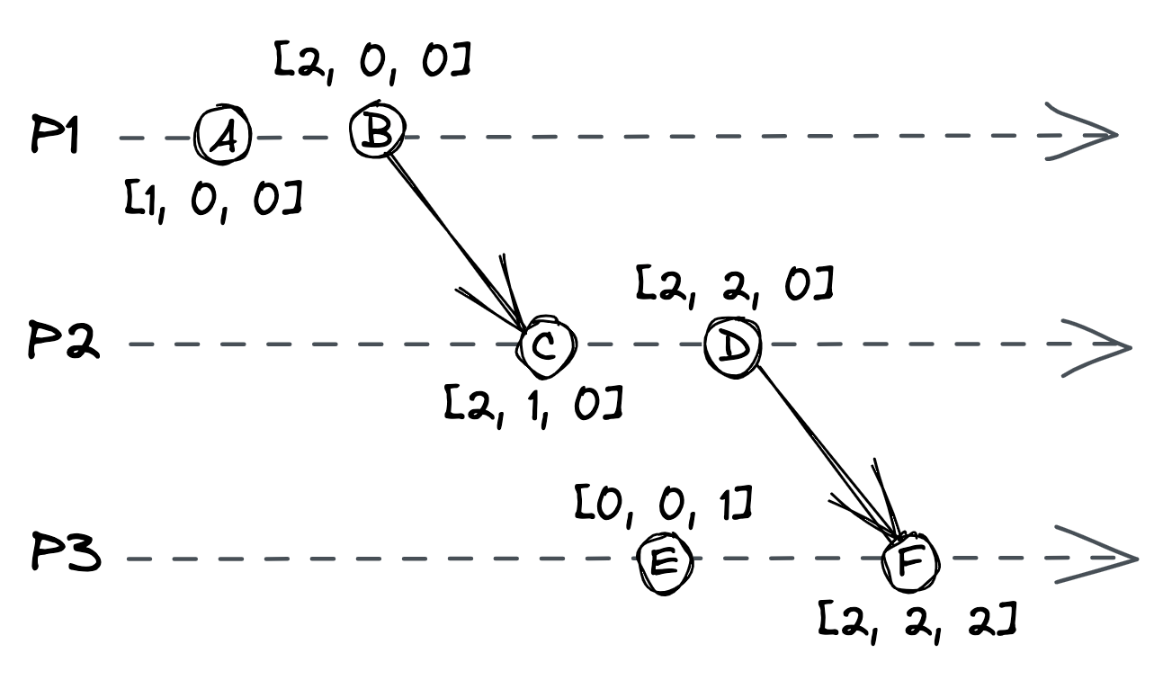
Figure 8.2: Each process has a vector clock represented by an array of three counters.
- every counter in T1 is less than or equal to the corresponding counter in T2,
- and there is at least one counter in T1 that is strictly less than the corresponding counter in T2,
then O1 happened-before O2. For example, in Figure 8.2, B happened-before C.
If O1 didn’t happen-before O2 and O2 didn’t happen-before O1, then the timestamps can’t be ordered, and the operations are considered to be concurrent. So, for example, operations E and C in Figure 8.2 can’t be ordered, and therefore are concurrent.
One problem with vector clocks is that the storage requirement on each process grows linearly with the number of processes, which becomes a problem for applications with many clients. However, there are other types of logical clocks that solve this issue, like dotted version vectors[7].
This discussion about logical clocks might feel a bit abstract at this point but bear with me. Later in this learning path, we will encounter some practical applications of logical clocks. What’s important to internalize at this point is that, in general, we can’t use physical clocks to accurately derive the order of events that happened on different processes. That being said, sometimes physical clocks are good enough. For example, using physical clocks to timestamp logs may be fine if they are only used for debugging purposes.
Leader election
Video coming soon. Start with the reading below.
There are times when a single process in the system needs to have special powers, like accessing a shared resource or assigning work to others. To grant a process these powers, the system needs to elect a leader among a set of candidate processes, which remains in charge until it relinquishes its role or becomes otherwise unavailable. When that happens, the remaining processes can elect a new leader among themselves.
A leader election algorithm needs to guarantee that there is at most one leader at any given time and that an election eventually completes even in the presence of failures. These two properties are also referred to as safety and liveness, respectively, and they are general properties of distributed algorithms. Informally, safety guarantees that nothing bad happens and liveness that something good eventually does happen. In this lesson, we will explore how a specific algorithm, the Raft leader election algorithm, guarantees these properties.
Raft leader election
Raft[1]’s leader election algorithm is implemented as a state machine in which any process is in one of three states (see Figure 9.1):
- the follower state, where the process recognizes another one as the leader;
- the candidate state, where the process starts a new election proposing itself as a leader;
- or the leader state, where the process is the leader.
In Raft, time is divided into election terms of arbitrary length that are numbered with consecutive integers (i.e., logical timestamps). A term begins with a new election, during which one or more candidates attempt to become the leader. The algorithm guarantees that there is at most one leader for any term. But what triggers an election in the first place?
When the system starts up, all processes begin their journey as followers. A follower expects to receive a periodic heartbeat from the leader containing the election term the leader was elected in. If the follower doesn’t receive a heartbeat within a certain period of time, a timeout fires and the leader is presumed dead. At that point, the follower starts a new election by incrementing the current term and transitioning to the candidate state. It then votes for itself and sends a request to all the processes in the system to vote for it, stamping the request with the current election term.
The process remains in the candidate state until one of three things happens: it wins the election, another process wins the election, or some time goes by with no winner:
- The candidate wins the election — The candidate wins the election if the majority of processes in the system vote for it. Each process can vote for at most one candidate in a term on a first-come-first-served basis. This majority rule enforces that at most one candidate can win a term. If the candidate wins the election, it transitions to the leader state and starts
sending heartbeats to the other processes. • Another process wins the election — If the candidate receives a heartbeat from a process that claims to be the leader with a term greater than or equal to the candidate’s term, it accepts the new leader and returns to the follower state.[2] If not, it continues in the candidate state. You might be wondering how that could happen; for example, if the candidate process was to stop for any reason, like for a long garbage collection pause, by the time it resumes another process could have won the election. • A period of time goes by with no winner — It’s unlikely but possible that multiple followers become candidates simultaneously, and none manages to receive a majority of votes; this is referred to as a split vote. The candidate will eventually time out and start a new election when that happens. The election timeout is picked randomly from a fixed interval to reduce the likelihood of another split vote in the next election.
Practical considerations
There are other leader election algorithms out there, but Raft’s implementation is simple to understand and also widely used in practice, which is why I chose it for this module. In practice, you will rarely, if ever, need to implement leader election from scratch. A good reason for doing that would be if you needed a solution with zero external dependencies[3]. Instead, you can use any fault-tolerant key-value store that offers a linearizable[4] compare-and-swap[5] operation with an expiration time (TTL).
The compare-and-swap operation atomically updates the value of a key if and only if the process attempting to update the value correctly identifies the current value. The operation takes three pa-
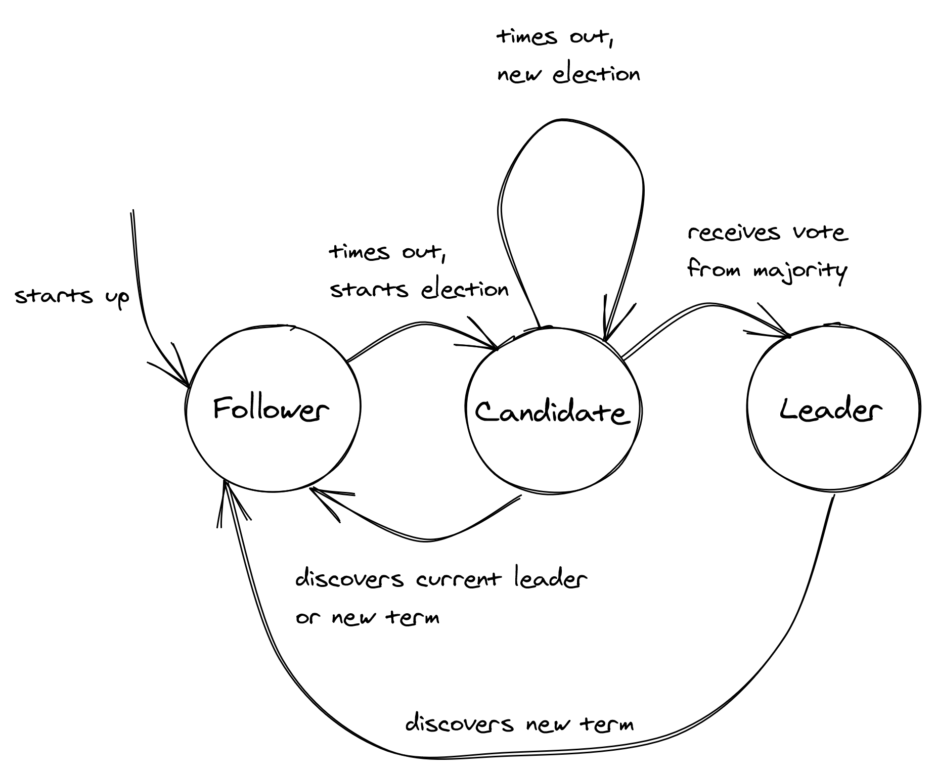
Figure 9.1: Raft’s leader election algorithm represented as a state machine.
rameters: K, Vo, and Vn, where Kis a key, and Voand Vnare values referred to as the old and new value, respectively. The operation atomically compares the current value of Kwith Vo, and if they match, it updates the value of Kto Vn. If the values don’t match, then Kis not modified, and the operation fails.
The expiration time defines the time to live for a key, after which the key expires and is removed from the store unless the expiration time is extended. The idea is that each competing process tries to acquire a lease by creating a new key with compare-and-swap. The first process to succeed becomes the leader and remains such until it stops renewing the lease, after which another process can become the leader.
The expiration logic can also be implemented on the client side, like this locking library[6] for DynamoDB does, but the implementation is more complex, and it still requires the data store to offer a compare-and-swap operation.
You might think that’s enough to guarantee there can’t be more than one leader at any given time. But, unfortunately, that’s not the case. To see why suppose multiple processes need to update a file on a shared file store, and we want to guarantee that only one at a time can access it to avoid race conditions. Now, suppose we use a lease to lock the critical section. Each process tries to acquire the lease, and the one that does so successfully reads the file, updates it in memory, and writes it back to the store:
if lease.acquire():
    try:
        content = store.read(filename)
        new_content = update(content)
        store.write(filename, new_content)
    except:
        lease.release()
The issue is that by the time the process gets to write to the file, it might no longer hold the lease. For example, the operating system might have preempted and stopped the process for long enough for the lease to expire. The process could try to detect that by comparing the lease expiration time to its local clock before writing to the store, assuming clocks are synchronized.
However, clock synchronization isn’t perfectly accurate. On top of that, the lease could expire while the request to the store is in-flight because of a network delay. To account for these problems, the process could check that the lease expiration is far enough in the future before writing to the file. Unfortunately, this workaround isn’t foolproof, and the lease can’t guarantee mutual exclusion by itself.
To solve this problem, we can assign a version number to each file that is incremented every time the file is updated. The process holding the lease can then read the file and its version number from the file store, do some local computation, and finally update the file (and increment the version number) conditional on the version number not having changed. The process can perform this validation atomically using a compare-and-swap operation, which many file stores support.
If the file store doesn’t support conditional writes, we have to design around the fact that occasionally there will be a race condition. Sometimes, that’s acceptable; for example, if there are momentarily two leaders and they both perform the same idempotent update, no harm is done.
Although having a leader can simplify the design of a system as it eliminates concurrency, it can also become a scalability bottleneck if the number of operations performed by it increases to the point where it can no longer keep up. Also, a leader is a single point of failure with a large blast radius; if the election process stops working or the leader isn’t working as expected, it can bring down the entire system with it. We can mitigate some of these downsides by introducing partitions and assigning a different leader per partition, but that comes with additional complexity. This is the solution many distributed data stores use since they need to use partitioning anyway to store data that doesn’t fit in a single node.
As a rule of thumb, if we must have a leader, we have to minimize the work it performs and be prepared to occasionally have more than one.
Taking a step back, a crucial assumption we made earlier is that the data store that holds leases is fault-tolerant, i.e., it can tolerate the loss of a node. Otherwise, if the data store ran on a single node and that node were to fail, we wouldn’t be able to acquire leases. For the data store to withstand a node failing, it needs to replicate its state over multiple nodes. In Replication (lesson 03.06), we will take a closer look at how this can be accomplished.
Replication
Video coming soon. Start with the reading below.
Data replication is a fundamental building block of distributed systems. One reason for replicating data is to increase availability. If some data is stored exclusively on a single process, and that process goes down, the data won’t be accessible anymore. However, if the data is replicated, clients can seamlessly switch to a copy. Another reason for replication is to increase scalability and performance; the more replicas there are, the more clients can access the data concurrently.
Implementing replication is challenging because it requires keeping replicas consistent with one another even in the face of failures. In this lesson, we will explore Raft’s replication algorithm[1], a replication protocol that provides the strongest consistency guarantee possible — the guarantee that to the clients, the data appears to be stored on a single process, even if it’s actually replicated. Arguably, the most popular protocol that offers this guarantee is Paxos[2], but we will discuss Raft as it’s more understandable.
Raft is based on a mechanism known as state machine replication. The main idea is that a single process, the leader, broadcasts operations that change its state to other processes, the followers (or replicas). If the followers execute the same sequence of operations as the leader, then each follower will end up in the same state as the leader. Unfortunately, the leader can’t simply broadcast operations to the followers and call it a day, as any process can fail at any time, and the network can lose messages. This is why a large part of the algorithm is dedicated to fault tolerance.
The reason why this mechanism is called stated machine replication is that each process is modeled as a state machine[3] that transitions from one state to another in response to some input (an operation). If the state machines are deterministic and get exactly the same input in the same order, their states are consistent. That way, if one of them fails, a redundant copy is available from any of the other state machines. State machine replication is a very powerful tool to make a service fault-tolerant as long it can be modeled as a state machine.
For example, consider the problem of implementing a fault-tolerant key-value store. In this case, each state machine represents a storage node that accepts put(k, v) and get(k) operations. The actual state is represented with a dictionary. When a put operation is executed, the key-value pair is added to the dictionary. When a get operation is executed, the value corresponding to the requested key is returned. You can see how if every node executes the same sequence of puts, all nodes will end up having the same state.
In the next section, we will take a deeper look at Raft’s replication protocol. It’s a challenging read that requires to pause and think, but I can assure you it’s well worth the effort, especially if you haven’t seen a replication protocol before.
State machine replication
When the system starts up, a leader is elected using Raft’s leader election algorithm discussed in Leader election (lesson 03.05), which doesn’t require any external dependencies. The leader is the only process that can change the replicated state. It does so by storing the sequence of operations that alter the state into a local log, which it replicates to the followers. Replicating the log is what allows the state to be kept in sync across processes.
As shown in Figure 10.1, a log is an ordered list of entries where each entry includes:
- the operation to be applied to the state, like the assignment of 3 to x. The operation needs to be deterministic so that all followers end up in the same state, but it can be arbitrarily complex as long as that requirement is respected (e.g., compareand-swap or a transaction with multiple operations);
- the index of the entry’s position in the log;
- and the leader’s election term (the number in each box).
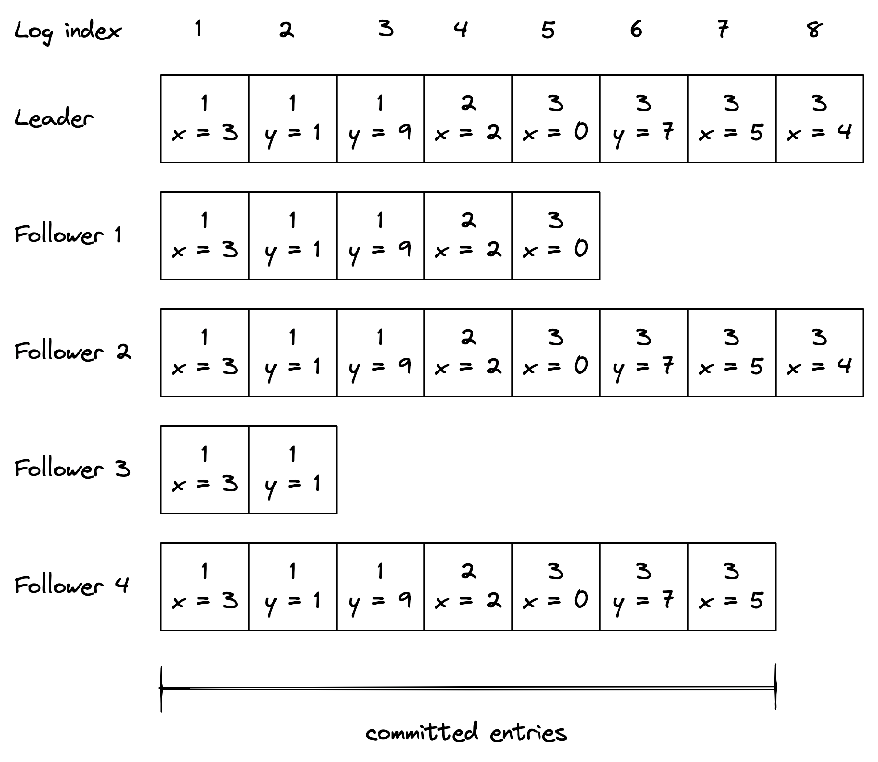
Figure 10.1: The leader’s log is replicated to its followers.
When the leader wants to apply an operation to its local state, it first appends a new entry for the operation to its log. At this point, the operation hasn’t been applied to the local state just yet; it has only been logged.
The leader then sends an AppendEntries request to each follower with the new entry to be added. This message is also sent out periodically, even in the absence of new entries, as it acts as a heartbeat for the leader.
When a follower receives an AppendEntries request, it appends the entry it received to its own log (without actually executing the operation yet) and sends back a response to the leader to acknowledge that the request was successful. When the leader hears back successfully from a majority of followers, it considers the entry to be committed and executes the operation on its local state. The leader keeps track of the highest committed index in the log, which is sent in all future AppendEntries requests. A follower only applies a log entry to its local state when it finds out that the leader has committed the entry.
Because the leader needs to wait for only a majority (quorum) of followers, it can make progress even if some are down, i.e., if there are 2f+ 1 followers, the system can tolerate up to ffailures. The algorithm guarantees that an entry that is committed is durable and will eventually be executed by all the processes in the system, not just those that were part of the original majority.
So far, we have assumed there are no failures, and the network is reliable. Let’s relax those assumptions. If the leader fails, a follower is elected as the new leader. But, there is a caveat: because the replication algorithm only needs a majority of processes to make progress, it’s possible that some processes are not up to date when a leader fails. To avoid an out-of-date process becoming the leader, a process can’t vote for one with a less up-to-date log. In other words, a process can’t win an election if it doesn’t contain all committed entries.
To determine which of two processes’ logs is more up-to-date, the election term and index of their last entries are compared. If the logs end with different terms, the log with the higher term is more up to date. If the logs end with the same term, whichever log is longer is more up to date. Since the election requires a majority vote, and a candidate’s log must be at least as up to date as any other process in that majority to win the election, the elected process will contain all committed entries.
If an AppendEntries request can’t be delivered to one or more followers, the leader will retry sending it indefinitely until a majority of the followers have successfully appended it to their logs. Retries are harmless as AppendEntries requests are idempotent, and followers ignore log entries that have already been appended to their logs.
If a follower that was temporarily unavailable comes back online, it will eventually receive an AppendEntries message with a log entry from the leader. The AppendEntries message includes the index and term number of the entry in the log that immediately precedes the one to be appended. If the follower can’t find a log entry with that index and term number, it rejects the message to prevent creating a gap in its log.
When the AppendEntries request is rejected, the leader retries the request, this time including the last two log entries — this is why we referred to the request as AppendEntries and not as AppendEntry. If that fails, the leader retries sending the last three log entries and so forth.[4] The goal is for the leader to find the latest log entry where the two logs agree, delete any entries in the follower’s log after that point, and append to the follower’s log all of the leader’s entries after it.
Consensus
By solving state machine replication, we actually found a solution to consensus[5] — a fundamental problem studied in distributed systems research in which a group of processes has to decide a value so that:
- every non-faulty process eventually agrees on a value;
- the final decision of every non-faulty process is the same everywhere;
- and the value that has been agreed on has been proposed by a process.
This may sound a little bit abstract. Another way to think about consensus is as the API of a write-once register[6] (WOR): a thread-safe and linearizable[7] register that can only be written once but can be read many times.
There are plenty of practical applications of consensus. For example, agreeing on which process in a group can acquire a lease requires consensus. And, as mentioned earlier, state machine replication also requires it. If you squint a little, you should be able to see how the replicated log in Raft is a sequence of WORs, and so Raft really is just a sequence of consensus instances.
While it’s important to understand what consensus is and how it can be solved, you will likely never need to implement it from scratch8. Instead, you can use one of the many off-the-shelf solutions available.
For example, one of the most common uses of consensus is for coordination purposes, like the election of a leader. As discussed in 9.2, leader election can be implemented by acquiring a lease. The lease ensures that at most one process can be the leader at any time and if the process dies, another one can take its place. However, this mechanism requires the lease manager, or coordination service, to be fault-tolerant. Etcd[9] and ZooKeeper[10] are two widely used coordination services that replicate their state for fault-tolerance using consensus. A coordination service exposes a hierarchical, keyvalue store through its API, and also allows clients to watch for changes to keys. So, for example, acquiring a lease can be implemented by having a client attempt to create a key with a specific TTL. If the key already exists, the operation fails guaranteeing that only one client can acquire the lease.
Consistency models
We discussed state machine replication with the goal of implementing a data store that can withstand failures and scale out to serve a larger number of requests. Now that we know how to build a replicated data store in principle, let’s take a closer look at what happens when a client sends a request to it. In an ideal world, the request executes instantaneously, as shown in Figure 10.2.
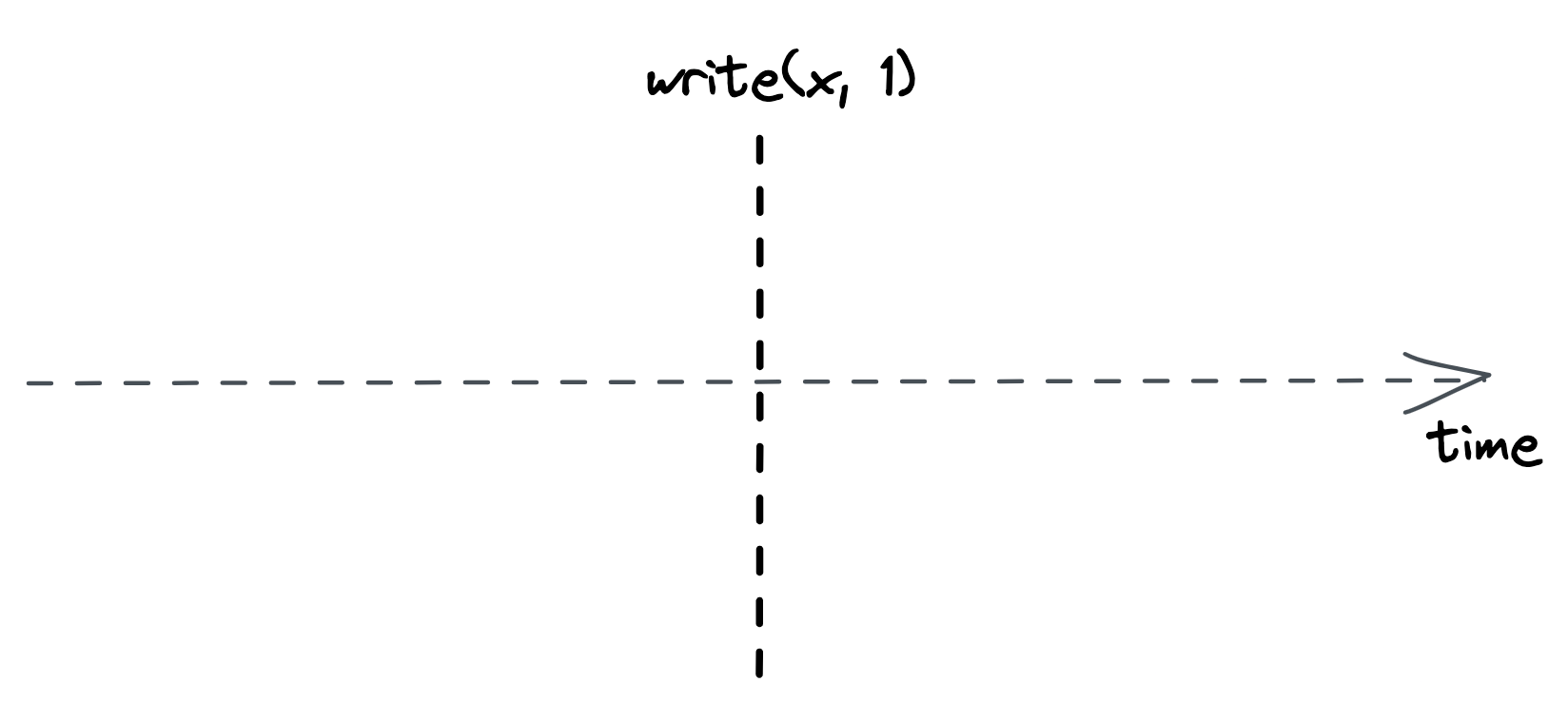
Figure 10.2: A write request executing instantaneously
But in reality, things are quite different — the request needs to reach the leader, which has to process it and send back a response to the client. As shown in Figure 10.3, these actions take time and are not instantaneous.
The best guarantee the system can provide is that the request executes somewhere between its invocation and completion time. You might think that this doesn’t look like a big deal; after all, it’s
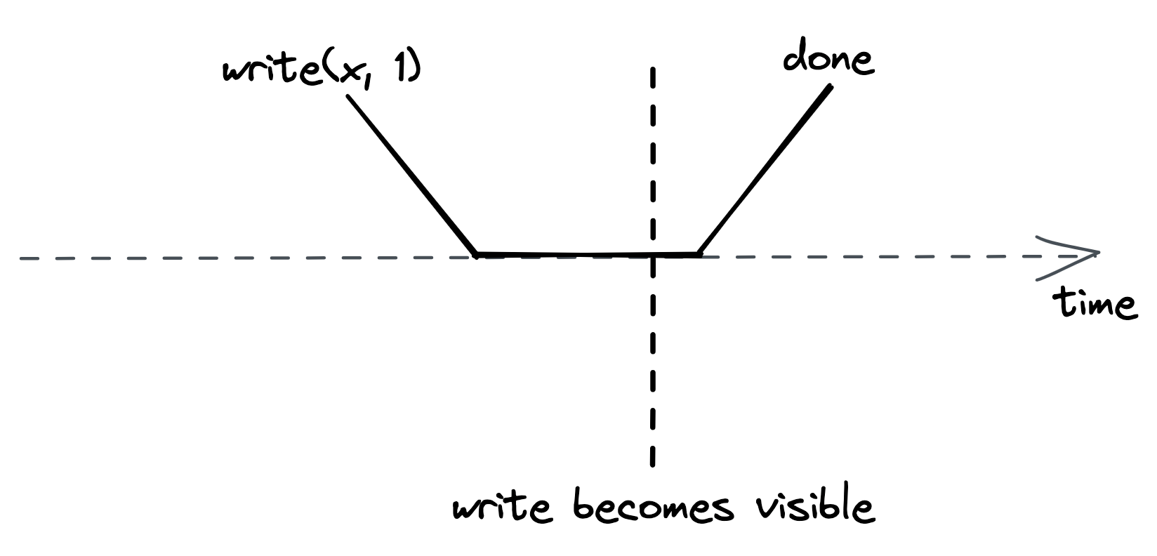
Figure 10.3: A write request can’t execute instantaneously because it takes time to reach the leader and be executed.
what you are used to when writing single-threaded applications. For example, if you assign 42 to x and read its value immediately afterward, you expect to find 42 in there, assuming there is no other thread writing to the same variable. But when you deal with replicated systems, all bets are off. Let’s see why that’s the case.
In State machine replication in Replication, we looked at how Raft replicates the leader’s state to its followers. Since only the leader can make changes to the state, any operation that modifies it needs to necessarily go through the leader. But what about reads? They don’t necessarily have to go through the leader as they don’t affect the system’s state. Reads can be served by the leader, a follower, or a combination of leader and followers. If all reads have to go through the leader, the read throughput would be limited to that of a single process. But, if any follower can serve reads instead, then two clients, or observers, can have a different view of the system’s state since followers can lag behind the leader.
Intuitively, there is a tradeoff between how consistent the observers’ views of the system are and the system’s performance and availability. To understand this relationship, we need to define precisely what we mean by consistency. We will do so with the help of consistency models[11], which formally define the possible views the observers can have of the system’s state.
Strong consistency
If clients send writes and reads exclusively to the leader, then every request appears to take place atomically at a very specific point in time as if there were a single copy of the data. No matter how many replicas there are or how far behind they are lagging, as long as the clients always query the leader directly, there is a single copy of the data from their point of view.
Because a request is not served instantaneously, and there is a single process that can serve it, the request executes somewhere between its invocation and completion time. By the time it completes, its side-effects are visible to all observers, as shown in Figure 10.4.
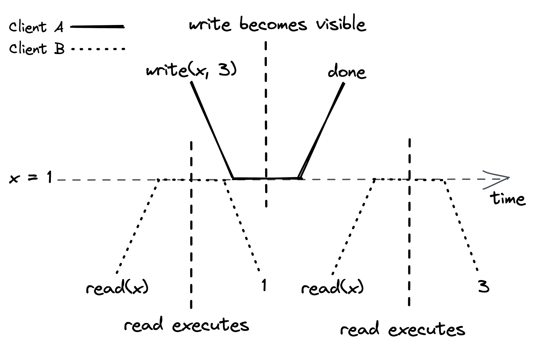
Figure 10.4: The side-effects of a strongly consistent operation are visible to all observers once it completes.
Since a request becomes visible to all other participants between its invocation and completion time, a real-time guarantee must be enforced; this guarantee is formalized by a consistency model called linearizability[12], or strong consistency. Linearizability is the strongest consistency guarantee a system can provide for single-object requests.[13]
Unfortunately, the leader can’t serve reads directly from its local state because by the time it receives a request from a client, it might no longer be the leader; so, if it were to serve the request, the system wouldn’t be strongly consistent. The presumed leader first needs to contact a majority of replicas to confirm whether it still is the leader. Only then is it allowed to execute the request and send back a response to the client. Otherwise, it transitions to the follower state and fails the request. This confirmation step considerably increases the time required to serve a read.
Sequential consistency
So far, we have discussed serializing all reads through the leader. But doing so creates a single chokepoint, limiting the system’s throughput. On top of that, the leader needs to contact a majority of followers to handle a read, which increases the time it takes to process a request. To increase the read performance, we could also allow the followers to handle requests.
Even though a follower can lag behind the leader, it will always receive new updates in the same order as the leader. For example, suppose one client only ever queries follower 1, and another only ever queries follower 2. In that case, the two clients will see the state evolving at different times, as followers are not perfectly in sync (see Figure 10.5).
The consistency model that ensures operations occur in the same order for all observers, but doesn’t provide any real-time guarantee about when an operation’s side-effect becomes visible to them, is called sequential consistency[14]. The lack of real-time guarantees is
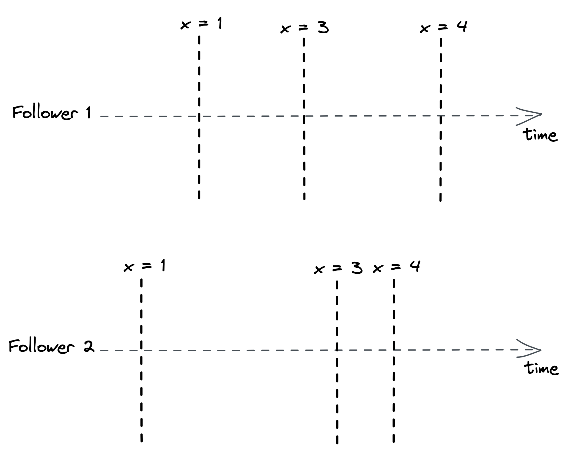
Figure 10.5: Although followers have a different view of the system’s state, they process updates in the same order.
what differentiates sequential consistency from linearizability.
A producer/consumer system synchronized with a queue is an example of this model; a producer writes items to the queue, which a consumer reads. The producer and the consumer see the items in the same order, but the consumer lags behind the producer.
Eventual consistency
Although we managed to increase the read throughput, we had to pin clients to followers — if a follower becomes unavailable, the client loses access to the store. We could increase the availability by allowing the client to query any follower. But this comes at a steep price in terms of consistency. For example, say there are two followers, 1 and 2, where follower 2 lags behind follower 1. If a client queries follower 1 and then follower 2, it will see an earlier state, which can be very confusing. The only guarantee the client has is that eventually all followers will converge to the final state if writes to the system stop. This consistency model is called eventual consistency.
It’s challenging to build applications on top of an eventually consistent data store because the behavior is different from what we are used to when writing single-threaded applications. As a result, subtle bugs can creep up that are hard to debug and reproduce. Yet, in eventual consistency’s defense, not all applications require linearizability. For example, an eventually consistent store is perfectly fine if we want to keep track of the number of users visiting a website, since it doesn’t really matter if a read returns a number that is slightly out of date.
The CAP theorem
When a network partition happens, parts of the system become disconnected from each other. For example, some clients might no longer be able to reach the leader. The system has two choices when this happens; it can either:
- remain available by allowing clients to query followers that are reachable, sacrificing strong consistency;
- or guarantee strong consistency by failing reads that can’t reach the leader.
This concept is expressed by the CAP theorem[15], which can be summarized as: “strong consistency, availability and partition tolerance: pick two out of three.” In reality, the choice really is only between strong consistency and availability, as network faults are a given and can’t be avoided.
Confusingly enough, the CAP theorem’s definition of availability requires that every request eventually receives a response. But in real systems, achieving perfect availability is impossible. Moreover, a very slow response is just as bad as one that never occurs. So, in other words, many highly-available systems can’t be considered available as defined by the CAP theorem. Similarly, the theorem’s definition of consistency and partition tolerance is very precise, limiting its practical applications.[16] A more useful way to think about the relationship between availability and consistency is as a spectrum. And so, for example, a strongly consistent and partition-tolerant system as defined by the CAP theorem occupies just one point in that spectrum.[17]
Also, even though network partitions can happen, they are usually rare within a data center. But, even in the absence of a network partition, there is a tradeoff between consistency and latency (or performance). The stronger the consistency guarantee is, the higher the latency of individual operations must be. This relationship is expressed by the PACELC theorem[18], an extension to the CAP theorem. It states that in case of network partitioning (P), one has to choose between availability (A) and consistency (C), but else (E), even when the system is running normally in the absence of partitions, one has to choose between latency (L) and consistency (C). In practice, the choice between latency and consistency is not binary but rather a spectrum.
This is why some off-the-shelf distributed data stores come with counter-intuitive consistency guarantees in order to provide high availability and performance. Others have knobs that allow you to choose whether you want better performance or stronger consistency guarantees, like Azure’s Cosmos DB[19] and Cassandra[20].
Another way to interpret the PACELC theorem is that there is a tradeoff between the amount of coordination required and performance. One way to design around this fundamental limitation is to move coordination away from the critical path. For example, earlier we discussed that for a read to be strongly consistent, the leader has to contact a majority of followers. That coordination tax is paid for each read! In the next section, we will explore a different replication protocol that moves this cost away from the critical path.
Chain replication
Chain replication[21] is a widely used replication protocol that uses a very different topology from leader-based replication protocols like Raft. In chain replication, processes are arranged in a chain. The leftmost process is referred to as the chain’s head, while the rightmost one is the chain’s tail.
Clients send writes exclusively to the head, which updates its local state and forwards the update to the next process in the chain. Similarly, that process updates its state and forwards the change to its successor until it eventually reaches the tail.
When the tail receives an update, it applies it locally and sends an acknowledgment to its predecessor to signal that the change has been committed. The acknowledgment flows back to the head, which can then reply to the client that the write succeeded[22].
Client reads are served exclusively by the tail, as shown in Fig 10.6. In the absence of failures, the protocol is strongly consistent as all writes and reads are processed one at a time by the tail. But what happens if a process in the chain fails?
Fault tolerance is delegated to a dedicated component, the configuration manager or control plane. At a high level, the control plane monitors the chain’s health, and when it detects a faulty process, it removes it from the chain. The control plane ensures that there is a
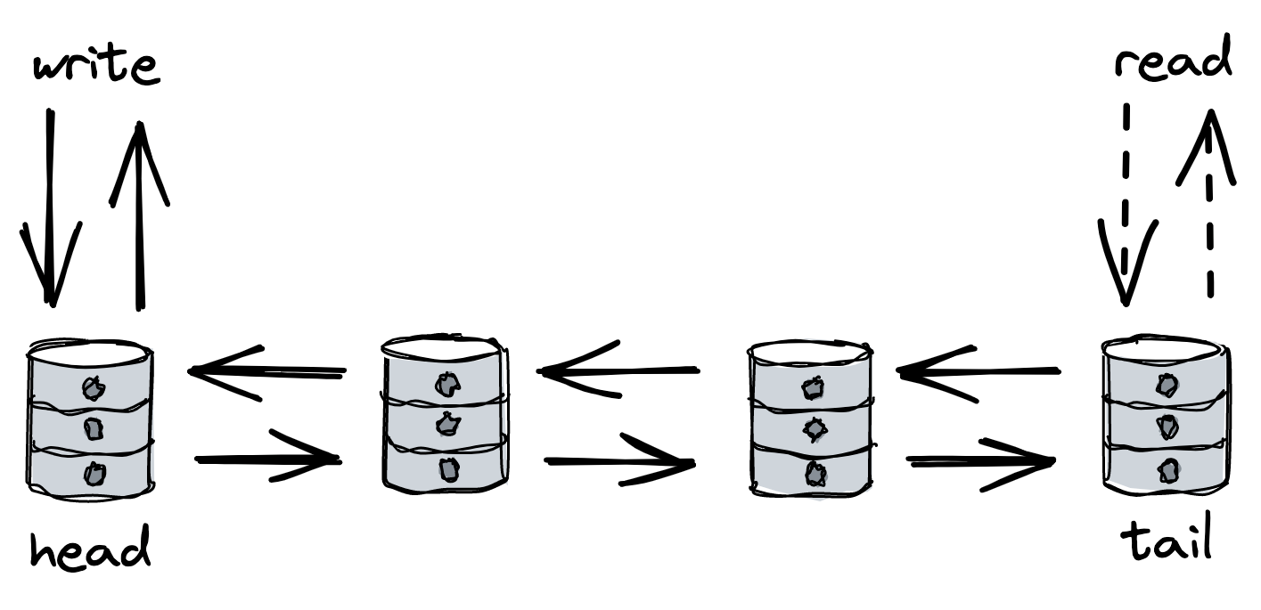
Figure 10.6: Writes propagate through all processes in the chain, while reads are served exclusively by the tail.
single view of the chain’s topology that every process agrees with. For this to work, the control plane needs to be fault-tolerant, which requires state machine replication (e.g., Raft). So while the chain can tolerate up to N −1 processes failing, where N is the chain’s length, the control plane can only tolerate C
2 failures, where C is the number of replicas that make up the control plane.
There are three failure modes in chain replication: the head can fail, the tail can fail, or an intermediate process can fail. If the head fails, the control plane removes it by reconfiguring its successor to be the new head and notifying clients of the change. If the head committed a write to its local state but crashed before forwarding it downstream, no harm is done. Since the write didn’t reach the tail, the client that issued it hasn’t received an acknowledgment for it yet. From the client’s perspective, it’s just a request that timed out and needs to be retried. Similarly, no other client will have seen the write’s side effects since it never reached the tail.
If the tail fails, the control plane removes it and makes its predecessor the chain’s new tail. Because all updates that the tail has received must necessarily have been received by the predecessor as well, everything works as expected.
If an intermediate process X fails, the control plane has to link X’s predecessor with X’s successor. This case is a bit trickier to handle since X might have applied some updates locally but failed before forwarding them to its successor. Therefore, X’s successor needs to communicate to the control plane the sequence number of the last committed update it has seen, which is then passed to X’s pre-decessor to send the missing updates downstream.
Chain replication can tolerate up to N −1 failures. So, as more processes in the chain fail, it can tolerate fewer failures. This is why it’s important to replace a failing process with a new one. This can be accomplished by making the new process the tail of the chain after syncing it with its predecessor.
The beauty of chain replication is that there are only a handful of simple failure modes to consider. That’s because for a write to commit, it needs to reach the tail, and consequently, it must have been processed by every process in the chain. This is very different from a quorum-based replication protocol like Raft, where only a subset of replicas may have seen a committed write.
Chain replication is simpler to understand and more performant than leader-based replication since the leader’s job of serving client requests is split among the head and the tail. The head sequences writes by updating its local state and forwarding updates to its successor. Reads, however, are served by the tail, and are interleaved with updates received from its predecessor. Unlike in Raft, a read request from a client can be served immediately from the tail’s local state without contacting the other replicas first, which allows for higher throughputs and lower response times.
However, there is a price to pay in terms of write latency. Since an update needs to go through all the processes in the chain before it can be considered committed, a single slow replica can slow down all writes. In contrast, in Raft, the leader only has to wait for a majority of processes to reply and therefore is more resilient to transient degradations. Additionally, if a process isn’t available, chain replication can’t commit writes until the control plane detects the problem and takes the failing process out of the chain. In Raft instead, a single process failing doesn’t stop writes from being committed since only a quorum of processes is needed to make progress.
That said, chain replication allows write requests to be pipelined, which can significantly improve throughput. Moreover, read throughput can be further increased by distributing reads across replicas while still guaranteeing linearizability. The idea is for replicas to store multiple versions of an object, each including a version number and a dirty flag. Replicas mark an update as dirty as it propagates from the head to the tail. Once the tail receives it, it’s considered committed, and the tail sends an acknowledgment back along the chain. When a replica receives an acknowledgment, it marks the corresponding version as clean. Now, when a replica receives a read request for an object, it will immediately serve it if the latest version is clean. If not, it first contacts the tail to request the latest committed version (see Fig 10.7).
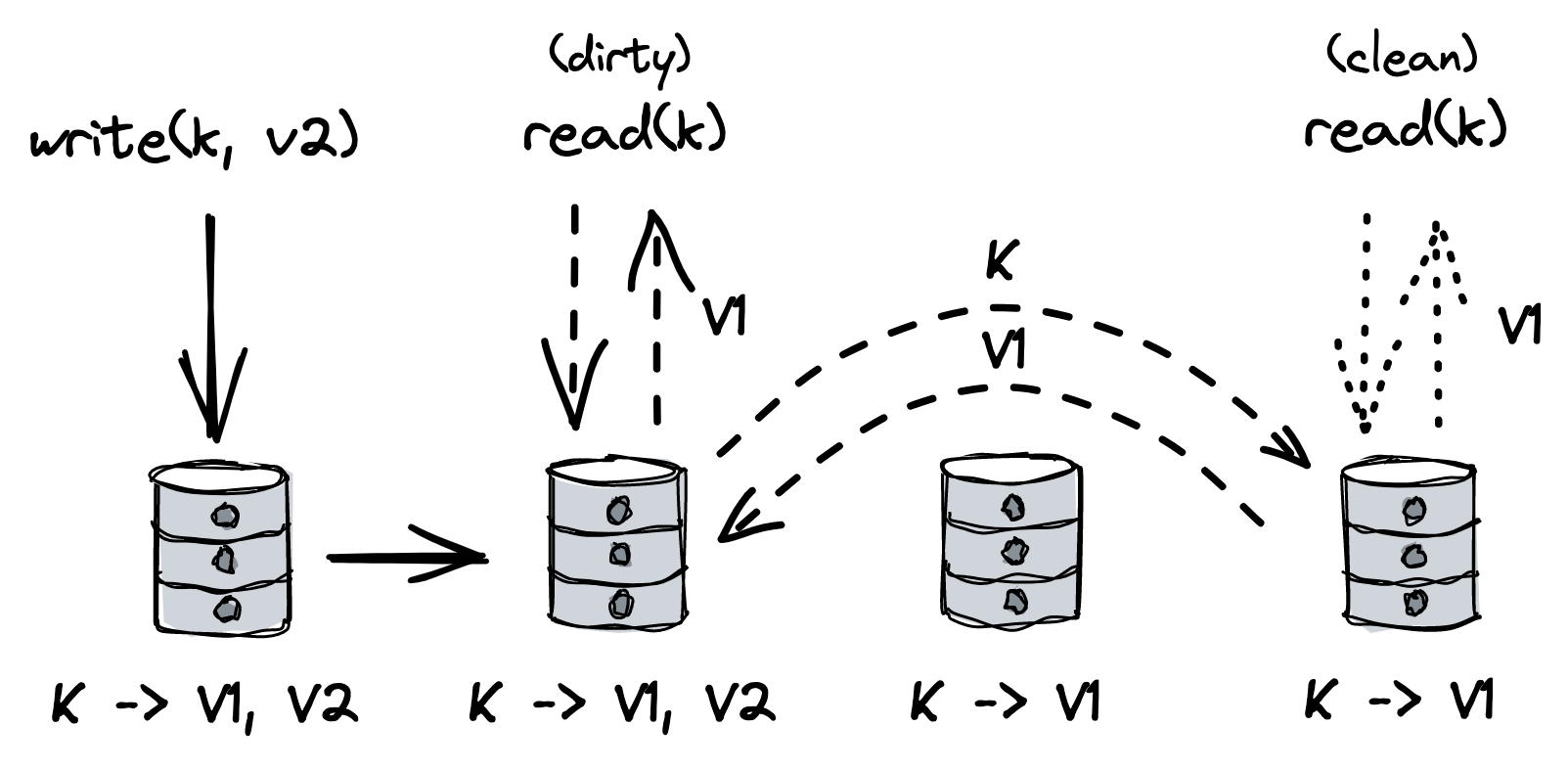
Figure 10.7: A dirty read can be served by any replica with an ad-ditional request to the tail to guarantee strong consistency.
As discussed in Leader election (lesson 03.05), a leader introduces a scalability bottleneck. But in chain replication, the data plane (i.e., the part of the system that handles individual client requests on the critical path) doesn’t need a leader to do its job since it’s not concerned with failures — its sole focus is throughput and efficiency. On the contrary, the control plane needs a leader to implement state machine replication, but that’s required exclusively to handle the occasional failure and doesn’t affect client requests on the critical path. Another way to think about this is that chain replication reduces the amount of coordination needed for each client request. In turn, this increases the data plane’s capacity to handle load. For this reason, splitting the data plane from the control plane (i.e., the configuration management part) is a common pattern in distributed systems. We will talk in more detail about this in Control planes and data planes (lesson 04.10).
You might be wondering at this point whether it’s possible to replicate data without needing consensus[23] at all to improve performance further. In Coordination avoidance (lesson 03.07), we will try to do just that.
Coordination avoidance
Video coming soon. Start with the reading below.
Another way of looking at state machine replication is as a system that requires two main ingredients:
- a broadcast protocol that guarantees every replica receives the same updates in the same order even in the presence of faults (aka fault-tolerant total order broadcast),
- and a deterministic function that handles updates on each replica.
Unsurprisingly, implementing a fault-tolerant total order broadcast protocol is what makes state machine replication hard to solve since it requires consensus[1]. More importantly, the need for a total order creates a scalability bottleneck since updates need to be processed sequentially by a single process (e.g., the leader in Raft). Also, total order broadcast isn’t available during network partitions as the CAP theorem applies[2] to it as well[3].
In this lesson, we will explore a form of replication that doesn’t require a total order but still comes with useful guarantees. But first, we need to talk about broadcast protocols.
Broadcast protocols
Network communication over wide area networks, like the internet, only offers point-to-point (unicast) communication protocols, like TCP. But to deliver a message to a group of processes, a broadcast protocol is needed (multicast). This means we have to somehow build a multicast protocol on top of a unicast one. The challenge here is that multicast needs to support multiple senders and receivers that can crash at any time.
A broadcast protocol is characterized by the guarantees it provides. Best-effort broadcast guarantees that if the sender doesn’t crash, the message is delivered to all non-faulty processes in a group. A simple way to implement it is to send the message to all processes in a group one by one over reliable links (see Fig 11.1). However, if, for example, the sender fails mid-way, some processes will never receive the message.
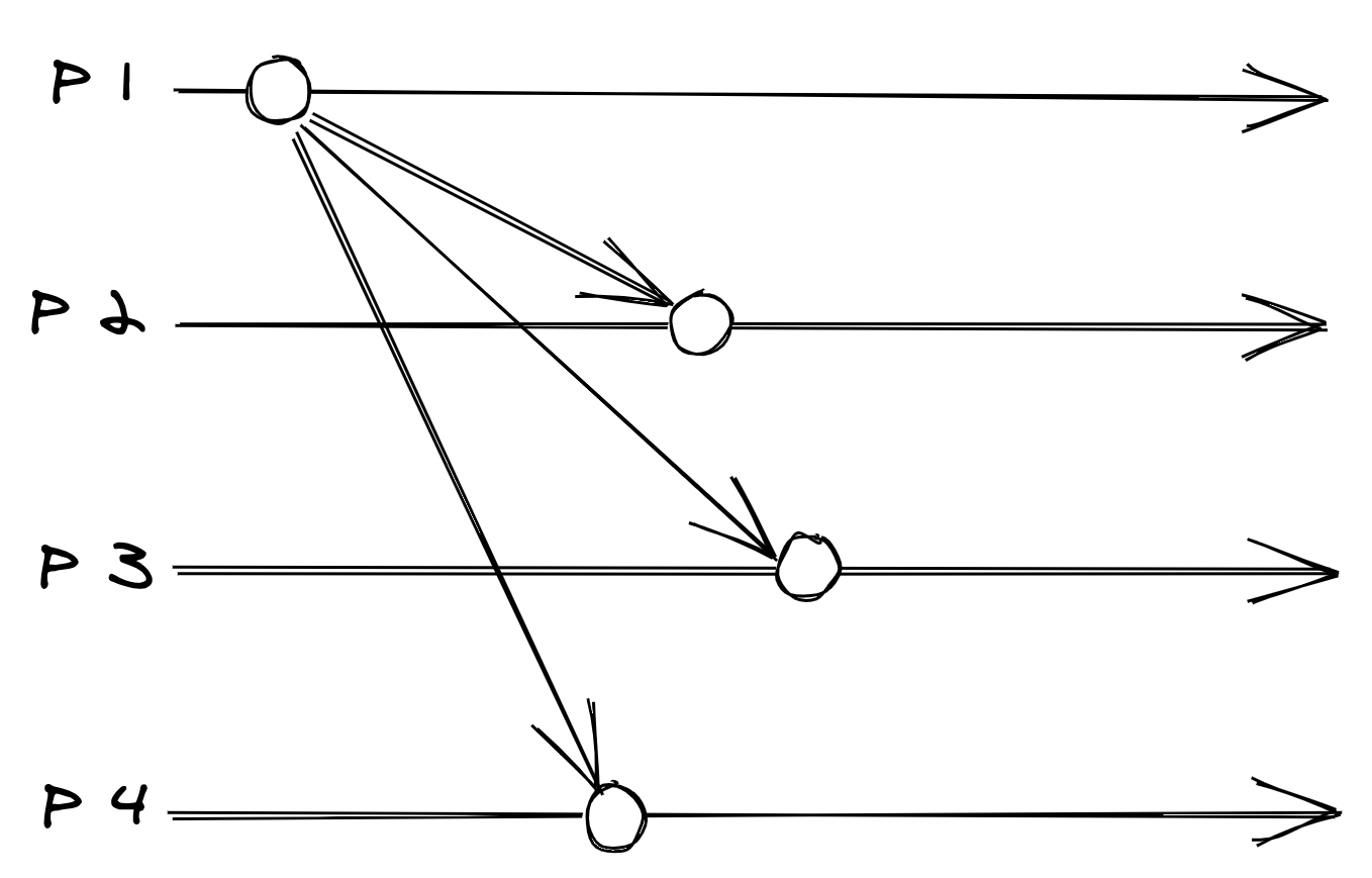
Figure 11.1: Best-effort broadcast
Unlike best-effort broadcast, reliable broadcast guarantees that the message is eventually delivered to all non-faulty processes in the group, even if the sender crashes before the message has been fully delivered. One way to implement reliable broadcast is to have each process retransmit the message to the rest of the group the first time it is delivered (see Fig 11.2). This approach is also known as eager reliable broadcast. Although it guarantees that all non-faulty processes eventually receive the message, it’s costly as it requires sending the message N[2] times for a group of Nprocesses.
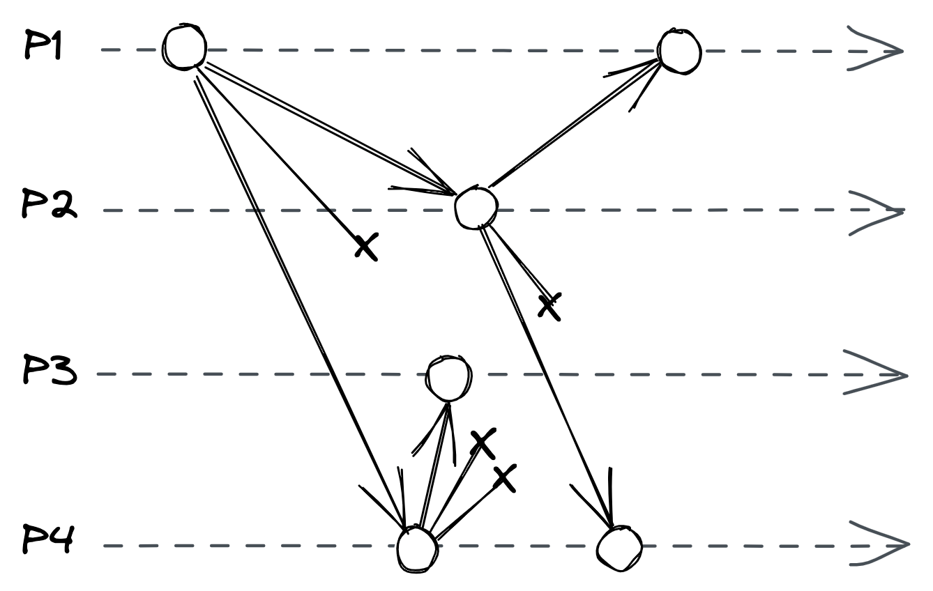
Figure 11.2: Eager reliable broadcast
The number of messages can be reduced by retransmitting a message only to a random subset of processes (e.g., 2 as in Fig 11.3). This implementation is referred to as a gossip broadcast protocol[4] as it resembles how rumors spread. Because it’s a probabilistic protocol, it doesn’t guarantee that a message will be delivered to all processes. That said, it’s possible to make that probability negligible by tuning the protocol’s parameters. Gossip protocols are particularly useful when broadcasting to a large number of processes where a deterministic protocol just wouldn’t scale.
Although reliable broadcast protocols guarantee that messages are delivered to all non-faulty processes in a group, they don’t make any guarantees about their order. For example, two processes could receive the same messages but in a different order. Total order broadcast is a reliable broadcast abstraction that builds upon the guarantees offered by reliable broadcast and additionally
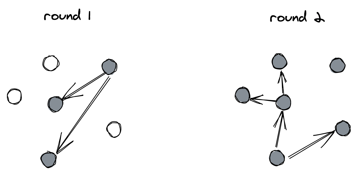
Figure 11.3: Gossip broadcast
ensures that messages are delivered in the same order to all processes. As discussed earlier, a fault-tolerant implementation requires consensus.
Conflict-free replicated data types
Now, here’s an idea: if we were to implement replication with a broadcast protocol that doesn’t guarantee total order, we wouldn’t need to serialize writes through a single leader, but instead could allow any replica to accept writes. But since replicas might receive messages in different orders, they will inevitably diverge. So, for the replication to be useful, the divergence can only be temporary, and replicas eventually have to converge to the same state. This is the essence of eventual consistency.
More formally, eventual consistency requires:
- eventual delivery — the guarantee that every update applied at a replica is eventually applied at all replicas,
- and convergence — the guarantee that replicas that have applied the same updates eventually reach the same state.
Using a broadcast protocol that doesn’t deliver messages in the same order across all replicas will inevitably lead to divergence
(see Fig 11.4). One way to reconcile conflicting writes is to use consensus to make a decision that all replicas need to agree with.
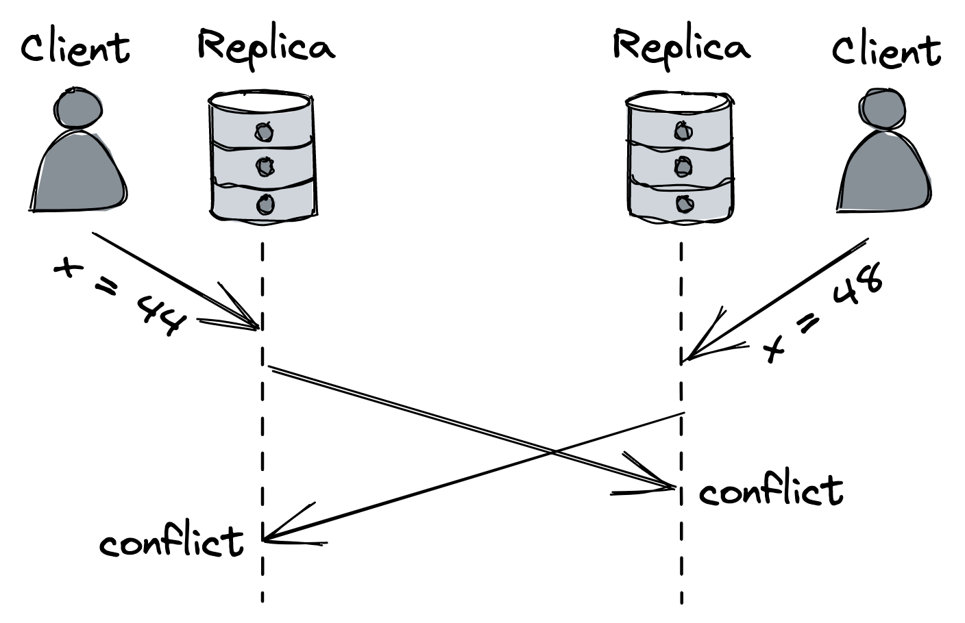
Figure 11.4: The same object is updated simultaneously by different clients at different replicas, leading to conflicts.
This solution has better availability and performance than the one using total order broadcast, since consensus is only required to reconcile conflicts and can happen off the critical path. But getting the reconciliation logic right isn’t trivial. So is there a way for replicas to solve conflicts without using consensus at all?
Well, if we can define a deterministic outcome for any potential conflict (e.g., the write with the greatest timestamp always wins), there wouldn’t be any conflicts, by design. Therefore consensus wouldn’t be needed to reconcile replicas. Such a replication strategy offers stronger guarantees than plain eventual consistency, i.e.:
- eventual delivery — the same guarantee as in eventual consistency,
- and strong convergence — the guarantee that replicas that have executed the same updates have the same state (i.e., every update is immediately persisted).
This variation of eventual consistency is also called strong eventual consistency[5]. With it, we can build systems that are available, (strongly eventual) consistent, and also partition tolerant.
Which conditions are required to guarantee that replicas strongly converge? For example, suppose we replicate an object across N replicas, where the object is an instance of some data type that supports query and update operations (e.g., integer, string, set, etc.).
A client can send an update or query operation to any replica, and:
- when a replica receives a query, it immediately replies using the local copy of the object;
- when a replica receives an update, it first applies it to the local copy of the object and then broadcasts the updated object to all replicas;
- and when a replica receives a broadcast message, it merges the object in the message with its own.
It can be shown that each replica will converge to the same state if:
- the object’s possible states form a semilattice, i.e., a set that contains elements that can be partially ordered;
- and the merge operation returns the least upper bound between two objects’ states (and therefore is idempotent, commutative, and associative).
A data type that has these properties is also called a convergent replicated data type[6], which is part of the family of conflict-free replicated data types (CRDTs). This sounds a lot more complicated than it actually is.
For example, suppose we are working with integer objects (which can be partially ordered), and the merge operation takes the maximum of two objects (least upper bound). It’s easy to see how replicas converge to the global maximum in this case, even if requests are delivered out of order and/or multiple times across replicas.
Although we have assumed the use of a reliable broadcast protocol so far, replicas could even use an unreliable protocol to implement broadcast as long as they periodically exchange and merge their states to ensure that they eventually converge (aka an anti-entropy mechanism, we will see some examples in Dynamo-style data stores in Coordination avoidance). Of course, periodic state exchanges can be expensive if done naively.
There are many data types that are designed to converge when replicated, like registers, counters, sets, dictionaries, and graphs. For example, a register is a memory cell storing some opaque sequence of bytes that supports an assignment operation to overwrite its state. To make a register convergent, we need to define a partial order over its values and a merge operation. There are two common register implementations that meet these requirements: last-writer-wins (LWW) and multi-value (MV).
A last-writer-wins register associates a timestamp with every update to make updates totally orderable. The timestamp could be composed of a Lamport timestamp to preserve the happened-before relationship among updates and a replica identifier to ensure there are no ties. When a replica receives an update request from a client, it generates a new timestamp and updates the register’s state with that and the new value; finally, it broadcasts the state and timestamp to all replicas. When a replica receives a register state from a peer, it merges it with its local copy by taking the one with the greater timestamp and discarding the other (see Fig 11.5).
The main issue with LWW registers is that conflicting updates that happen concurrently are handled by taking the one with the greater timestamp, which might not always make sense. An alternative way of handling conflicts is to keep track of all concurrent updates and return them to the client application, which can handle conflicts however it sees fit. This is the approach taken by the multi-value register. To detect concurrent updates, replicas tag each update with a vector clock timestamp[7] and the merge
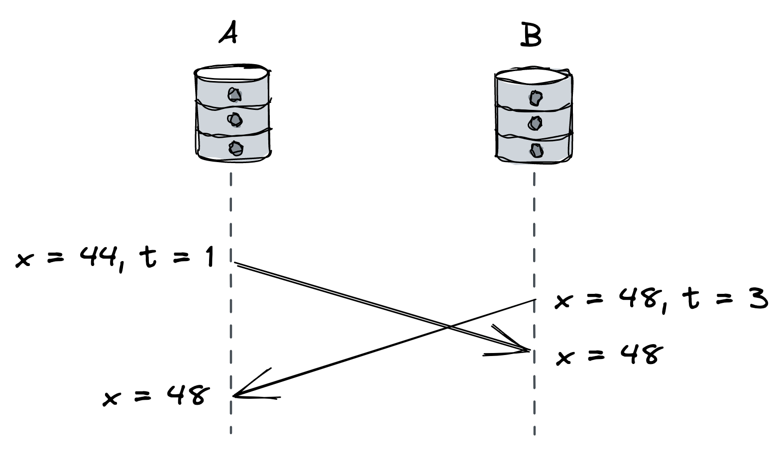
Figure 11.5: Last-writer wins register
operation returns the union of all concurrent updates (see Fig 11.6).
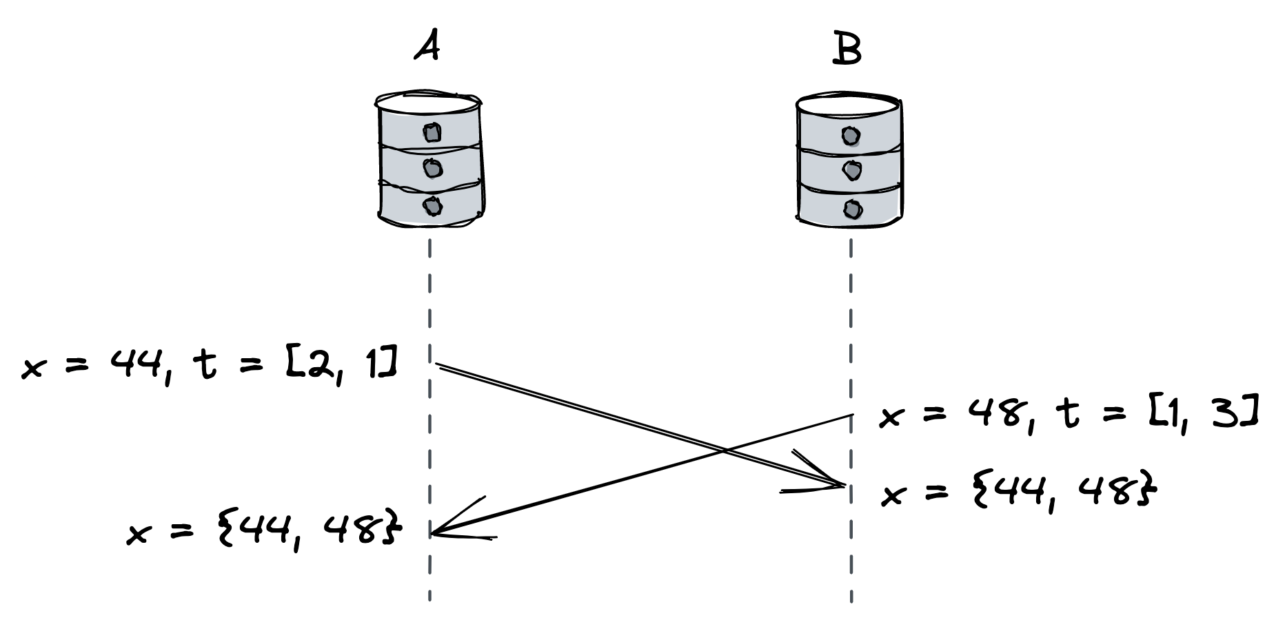
Figure 11.6: Multi-value register
The beauty of CRDTs is that they compose. So, for example, you can build a convergent key-value store by using a dictionary of LWW or MV registers. This is the approach followed by Dynamostyle data stores.
Dynamo-style data stores
Dynamo[8] is arguably the best-known design of an eventually consistent and highly available key-value store. Many other data stores have been inspired by it, like Cassandra[9] and Riak KV[10].
In Dynamo-style data stores, every replica can accept write and read requests. When a client wants to write an entry to the data store, it sends the request to all N replicas in parallel but waits for an acknowledgment from just W replicas (a write quorum). Similarly, when a client wants to read an entry from the data store, it sends the request to all replicas but waits just for R replies (a read quorum) and returns the most recent entry to the client. To resolve conflicts, entries behave like LWW or MV registers depending on the implementation flavor.
When W + R > N, the write quorum and the read quorum must intersect with each other, so at least one read will return the latest version (see Fig 11.7). This doesn’t guarantee linearizability on its own, though. For example, if a write succeeds on less than W replicas and fails on the others, replicas are left in an inconsistent state, and some clients might read the latest version while others don’t. To avoid this inconsistency, the writes need to be bundled into an atomic transaction. We will talk more about transactions in Transactions (lesson 03.08).
Typically W and R are configured to be majority quorums, i.e., quorums that contain more than half the number of replicas. That said, other combinations are possible, and the data store’s read and write throughput depend on how large or small R and W are. For example, a read-heavy workload benefits from a smaller R; however, this makes writes slower and less available (assuming W + R > N). Alternatively, both W and R can be configured to be very small (e.g., W = R = 1) for maximum performance at the expense of consistency (W + R < N).
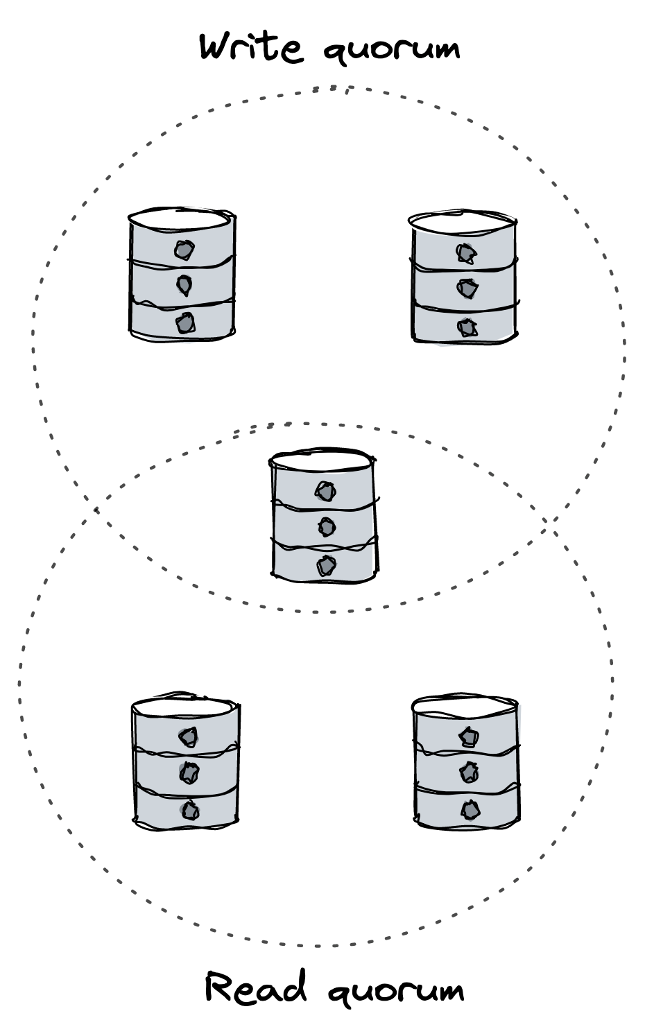
Figure 11.7: Intersecting write and read quorums
One problem with this approach is that a write request sent to a replica might never make it to the destination. In this case, the replica won’t converge, no matter how long it waits. To ensure that replicas converge, two anti-entropy mechanisms are used: read-repair and replica synchronization. So another way to think about quorum replication is as a best-effort broadcast combined with anti-entropy mechanisms to ensure that all changes propagate to all replicas.
Read repair is a mechanism that clients implement to help bring replicas back in sync whenever they perform a read. As mentioned earlier, when a client executes a read, it waits for R replies. Now, suppose some of these replies contain older entries. In that case, the client can issue a write request with the latest entry to the outof-sync replicas. Although this approach works well for frequently read entries, it’s not enough to guarantee that all replicas will eventually converge.
Replica synchronization is a continuous background mechanism that runs on every replica and periodically communicates with others to identify and repair inconsistencies. For example, suppose replica X finds out that it has an older version of key K than replica Y. In that case, it will retrieve the latest version of K from Y. To detect inconsistencies and minimize the amount of data exchanged, replicas can exchange Merkle tree hashes[11] with a gossip protocol.
The CALM theorem
At this point, you might be wondering how you can tell whether an application requires coordination, such as consensus, and when it doesn’t. The CALM theorem[12] states that a program has a consistent, coordination-free distributed implementation if and only if it is monotonic.
Intuitively, a program is monotonic if new inputs further refine the output and can’t take back any prior output. A program that computes the union of a set is a good example of that — once an element (input) is added to the set (output), it can’t be removed. Similarly, it can be shown that CRDTs are monotonic.
In contrast, in a non-monotonic program, a new input can retract a prior output. For example, variable assignment is a non-monotonic operation since it overwrites the variable’s prior value.
A monotonic program can be consistent, available, and partition tolerant all at once. However, consistency in CALM doesn’t refer to linearizability, the C in CAP. Linearizability is narrowly focused on the consistency of reads and writes. Instead, CALM focuses on the consistency of the program’s output[13]. In CALM, a consistent program is one that produces the same output no matter in which order the inputs are processed and despite any conflicts; it doesn’t say anything about the consistency of reads and writes.
For example, say you want to implement a counter. If all you have at your disposal are write and read operations, then the order of the operations matters:
write(1), write(2), write(3) => 3but:
write(3), write(1), write(2) => 2In contrast, if the program has an abstraction for counters that supports an increment operation, you can reorder the operations any way you like without affecting the result:
increment(1), increment(1), increment(1) => 3In other words, consistency based on reads and writes can limit the solution space[14], since it’s possible to build systems that are consistent at the application level, but not in terms of reads and writes at the storage level.
CALM also identifies programs that can’t be consistent because they are not monotonic. For example, a vanilla register/variable assignment operation is not monotonic as it invalidates whatever value was stored there before. But, by combining the assignment operation with a logical clock, it’s possible to build a monotonic implementation, as we saw earlier when discussing LWW and MV registers.
Causal consistency
So we understand now how eventual consistency can be used to implement monotonic applications that are consistent, available, and partition-tolerant. Unfortunately, there are many applications for which its guarantees are not sufficient. For example, eventual consistency doesn’t guarantee that an operation that happenedbefore another is observed in the correct order by replicas. Suppose you upload a picture to a social network and then add it to a gallery. With eventual consistency, the gallery may reference the image before it becomes available, causing a missing image placeholder to appear in its stead.
One of the main benefits of strong consistency is that it preserves the happened-before order among operations, which guarantees that the cause happens before the effect. So, in the previous example, the reference to the newly added picture in the gallery is guaranteed to become visible only after the picture becomes available.
Surprisingly, to preserve the happened-before order (causal order) among operations, we don’t need to reach for strong consistency, since we can use a weaker consistency model called causal consistency[15]. This model is weaker than strong consistency but stronger than eventual consistency, and it’s particularly attractive for two reasons:
- For many applications, causal consistency is “consistent enough” and easier to work with than eventual consistency.
- Causal consistency is provably[16] the strongest consistency model that enables building systems that are also available and partition tolerant.
Causal consistency imposes a partial order on the operations. The simplest definition requires that processes agree on the order of causally related operations but can disagree on the order of unrelated ones. You can take any two operations, and either one happened-before the other, or they are concurrent and therefore can’t be ordered. This is the main difference from strong consistency, which imposes a global order that all processes agree with.
For example, suppose a process updates an entry in a key-value store (operation A), which is later read by another process (operation B) that consequently updates another entry (operation C). In that case, all processes in the system have to agree that A happenedbefore C. In contrast, if two operations, X and Y, happen concurrently and neither happened-before the other, some processes may observe X before Y and others Y before X.
Let’s see how we can use causal consistency to build a replicated data store that is available under network partitions. We will base our discussion on “Clusters of Order-Preserving Servers” (COPS[17]), a key-value store that delivers causal consistency across geographically distributed clusters. In COPS, a cluster is set up as a strongly consistent partitioned data store, but for simplicity, we will treat it as a single logical node without partitions.[18] Later, in Partitioning (lesson 04.04), we will discuss partitioning at length.
First, let’s define a variant of causal consistency called causal+ in which there is no disagreement (conflict) about the order of unrelated operations. Disagreements are problematic since they cause replicas to diverge forever. To avoid them, LWW registers can be used as values to ensure that all replicas converge to the same state in the presence of concurrent writes. An LWW register is composed of an object and a logical timestamp, which represents its version.
In COPS, any replica can accept read and write requests, and clients send requests to their closest replica (local replica). When a client sends a read request for a key to its local replica, the latter replies with the most recent value available locally. When the client receives the response, it adds the version (logical timestamp) of the value it received to a local key-version dictionary used to keep track of dependencies.
When a client sends a write to its local replica, it adds a copy of the dependency dictionary to the request. The replica assigns a version to the write, applies the change locally, and sends an acknowledgment back to the client with the version assigned to it. It can apply the change locally, even if other clients updated the key in the meantime, because values are represented with LWW registers. Finally, the update is broadcast asynchronously to the other replicas.
When a replica receives a replication message for a write, it doesn’t apply it locally immediately. Instead, it first checks whether the write’s dependencies have been committed locally. If not, it waits until the required versions appear. Finally, once all dependencies have been committed, the replication message is applied locally. This behavior guarantees causal consistency (see Fig 11.8).
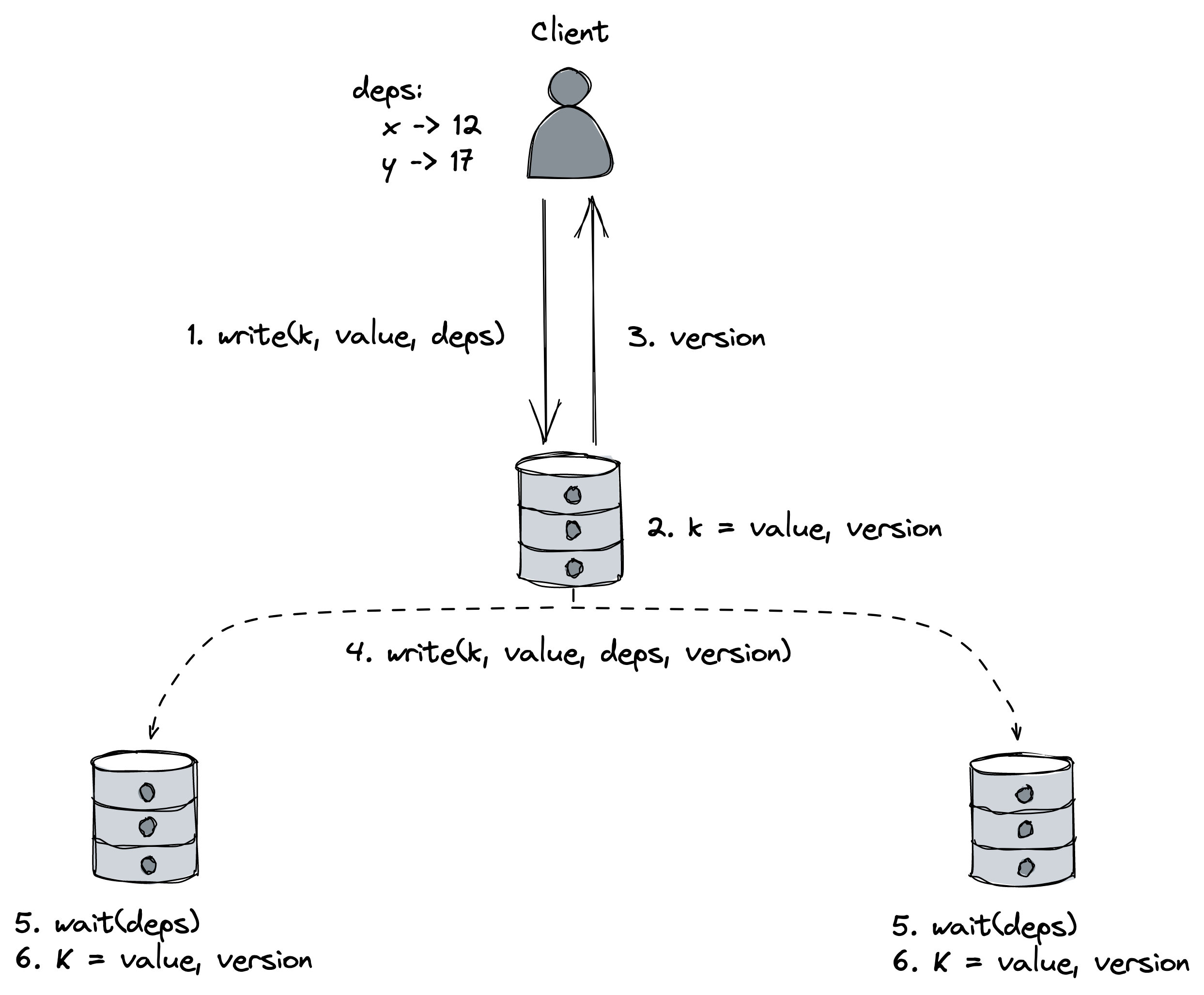
Figure 11.8: A causally consistent implementation of a key-value store
If a replica fails, the data store continues to be available as any replica can accept writes. There is a possibility that a replica could fail after committing an update locally but before broadcasting it, resulting in data loss. In COPS’ case, this tradeoff is considered acceptable to avoid paying the price of waiting for one or more long-distance requests to remote replicas before acknowledging a client write.
Practical considerations
To summarize, in the earlier lessons we explored different ways to implement replication and learned that there is a tradeoff between consistency and availability/performance. In other words, to build scalable and available systems, coordination needs to be minimized.
This tradeoff is present in any large-scale system, and some even have knobs that allow you to control it. For example, Azure Cosmos DB is a fully managed scalable NoSQL database that enables developers to choose among 5 different consistency models, ranging from eventual consistency to strong consistency[19], where weaker consistency models have higher throughputs than stronger ones.
Transactions
Video coming soon. Start with the reading below.
Transactions[1] provide the illusion that either all the operations within a group complete successfully or none of them do, as if the group were a single atomic operation. If you have used a relational database such as MySQL or PostgreSQL in the past, you should be familiar with the concept.
If your application exclusively updates data within a single relational database, then bundling some changes into a transaction is straightforward. On the other hand, if your system needs to atomically update data that resides in multiple data stores, the operations need to be wrapped into a distributed transaction, which is a lot more challenging to implement. This is a fairly common scenario in microservice architectures where a service needs to interact with other services to handle a request, and each service has its own separate data store. In this lesson, we explore various solutions to this problem.
ACID
Consider a money transfer from one bank account to another. If the withdrawal succeeds, but the deposit fails for some reason, the funds need to be deposited back into the source account. In other words, the transfer needs to execute atomically; either both the withdrawal and the deposit succeed, or in case of a failure, neither do. To achieve that, the withdrawal and deposit need to be wrapped in an inseparable unit of change: a transaction.
In a traditional relational database, a transaction is a group of operations for which the database guarantees a set of properties, known as ACID:
- Atomicity guarantees that partial failures aren’t possible; either all the operations in the transactions complete successfully, or none do. So if a transaction begins execution but fails for whatever reason, any changes it made must be undone. This needs to happen regardless of whether the transaction itself failed (e.g., divide by zero) or the database crashed mid way.
- Consistency guarantees that the application-level invariants must always be true. In other words, a transaction can only transition a database from a correct state to another correct state. How this is achieved is the responsibility of the application developer who defines the transaction. For example, in a money transfer, the invariant is that the sum of money across the accounts is the same after the transfer, i.e., money can’t be destroyed or created. Confusingly, the “C” in ACID has nothing to do with the consistency models we talked about so far, and according to Joe Hellerstein, it was tossed in to make the acronym work[2]. Therefore, we will safely ignore this property in the rest of the chapter.
- Isolation guarantees that a transaction appears to run in isolation as if no other transactions are executing, i.e., the concurrent execution of transactions doesn’t cause any race con-
ditions. • Durability guarantees that once the database commits the transaction, the changes are persisted on durable storage so that the database doesn’t lose the changes if it subsequently crashes. In the way I described it, it sounds like the job is done once the data is persisted to a storage device. But, we know better by now, and replication[3] is required to ensure durability in the presence of storage failures.
Transactions relieve developers from a whole range of possible failure scenarios so that they can focus on the actual application logic rather than handling failures. But to understand how distributed transactions work, we first need to discuss how centralized, non-distributed databases implement transactions.
Isolation
The easiest way to guarantee that no transaction interferes with another is to run them serially one after another (e.g., using a global lock). But, of course, that would be extremely inefficient, which is why in practice transactions run concurrently. However, a group of concurrently running transactions accessing the same data can run into all sorts of race conditions, like dirty writes, dirty reads, fuzzy reads, and phantom reads:
- A dirty write happens when a transaction overwrites the value written by another transaction that hasn’t committed yet.
- A dirty read happens when a transaction observes a write from a transaction that hasn’t completed yet.
- A fuzzy read happens when a transaction reads an object’s value twice but sees a different value in each read because another transaction updated the value between the two reads.
- A phantom read happens when a transaction reads a group of objects matching a specific condition, while another transaction concurrently adds, updates, or deletes objects match-
ing the same condition. For example, if one transaction is summing all employees’ salaries while another deletes some employee records simultaneously, the final sum will be incorrect at commit time.
To protect against these race conditions, a transaction needs to be isolated from others. An isolation level protects against one or more types of race conditions and provides an abstraction that we can use to reason about concurrency. The stronger the isolation level is, the more protection it offers against race conditions, but the less performant it is.
An isolation level is defined based on the type of race conditions it forbids, as shown in Figure 12.1.
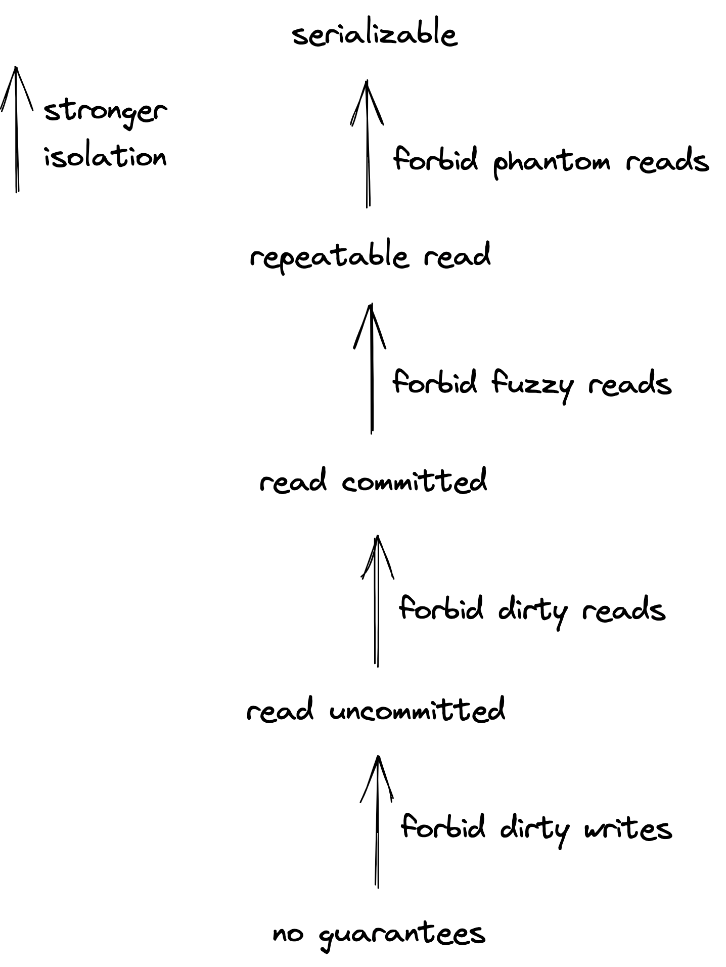
Figure 12.1: Isolation levels define which race conditions they forbid.
Serializability is the only isolation level that isolates against all possible race conditions. It guarantees that executing a group of transactions has the same side effects as if the transactions run serially (one after another) in some order. For example, suppose we have two concurrent transactions, X and Y, and transaction X commits before transaction Y. A serializable system guarantees that even though their operations are interleaved, they appear to run after the other, i.e., X before Y or Y before X (even if Y committed after!). To add a real-time requirement on the order of transactions, we need a stronger isolation level: strict serializability. This level combines serializability with the real-time guarantees of linearizability so that when a transaction completes, its side effects become immediately visible to all future transactions.
(Strict) serializability is slow as it requires coordination, which creates contention in the system. For example, a transaction may be forced to wait for other transactions. In some cases, it may even be forced to abort because it can no longer be executed as part of a serializable execution. Because not all applications require the guarantees that serializability provides, data stores allow developers to use weaker isolation levels. As a rule of thumb, we need to consciously decide which isolation level to use and understand its implications, or the data store will silently make that decision for us; for example, PostgreSQL’s default isolation[4] is read committed. So, if in doubt, choose strict serializability.
There are more isolation levels and race conditions than the ones we discussed here. Jepsen[5] provides a good formal reference for the existing isolation levels, how they relate to one another, and which guarantees they offer. Although vendors typically document the isolation levels of their products, these specifications don’t always match[6] the formal definitions.
Now that we know what serializability is, the challenge becomes maximizing concurrency while still preserving the appearance of serial execution. The concurrency strategy is defined by a concurrency control protocol, and there are two categories of protocols that guarantee serializability: pessimistic and optimistic.
Concurrency control
A pessimistic protocol uses locks to block other transactions from accessing an object. The most commonly used protocol is two-phase locking[7] (2PL). 2PL has two types of locks, one for reads and one for writes. A read lock can be shared by multiple transactions that access the object in read-only mode, but it blocks transactions trying to acquire a write lock. A write lock can be held only by a single transaction and blocks anyone trying to acquire either a read or write lock on the object. The locks are held by a lock manager that keeps track of the locks granted so far, the transactions that acquired them, and the transactions waiting for them to be released.
There are two phases in 2PL, an expanding phase and a shrinking one. In the expanding phase, the transaction is allowed only to acquire locks but not release them. In the shrinking phase, the transaction is permitted only to release locks but not acquire them. If these rules are obeyed, it can be formally proven that the protocol guarantees strict serializability. In practice, locks are only released when the transaction completes (aka strict 2PL). This ensures that data written by an uncommitted transaction X is locked until it’s committed, preventing another transaction Y from reading it and consequently aborting if X is aborted (aka cascading abort), resulting in wasted work.
Unfortunately, with 2PL, it’s possible for two or more transactions to deadlock and get stuck. For example, if transaction X is waiting for a lock that transaction Y holds, and transaction Y is waiting for a lock granted to transaction X, then the two transactions won’t make any progress. A general approach to deal with deadlocks is to detect them after they occur and select a “victim” transaction to abort and restart to break the deadlock.
In contrast to a pessimistic protocol, an optimistic protocol optimistically executes a transaction without blocking based on the assumption that conflicts are rare and transactions are short-lived. Optimistic concurrency control[8](OCC) is arguably the best-known protocol in the space. In OCC, a transaction writes to a local workspace without modifying the actual data store. Then, when the transaction wants to commit, the data store compares the transaction’s workspace to see whether it conflicts with the workspace of another running transaction. This is done by assigning each transaction a timestamp that determines its serializability order. If the validation succeeds, the content of the local workspace is copied to the data store. If the validation fails, the transaction is aborted and restarted.
It’s worth pointing out that OCC uses locks to guarantee mutual exclusion on internal shared data structures. These physical locks are held for a short duration and are unrelated to the logical locks we discussed earlier in the context of 2PL. For example, during the validation phase, the data store has to acquire locks to access the workspaces of the running transactions to avoid race conditions. In the database world, these locks are also referred to as latches to distinguish them from logical locks.
Optimistic protocols avoid the overhead of pessimistic protocols, such as acquiring locks and managing deadlocks. As a result, these protocols are well suited for read-heavy workloads that rarely perform writes or workloads that perform writes that only occasionally conflict with each other. On the other hand, pessimistic protocols are more efficient for conflict-heavy workloads since they avoid wasting work.
Taking a step back, both the optimistic and pessimistic protocols discussed this far aren’t optimal for read-only transactions. In 2PC, a read-only transaction might wait for a long time to acquire a shared lock. On the other hand, in OCC, a read-only transaction may be aborted because the value it read has been overwritten. Generally, the number of read-only transactions is much higher than the number of write transactions, so it would be ideal if a read-only transaction could never block or abort because of a conflict with a write transaction.
Multi-version concurrency control[9] (MVCC) delivers on that premise by maintaining older versions of the data. Conceptually, when a transaction writes an object, the data store creates a new version of it. And when the transaction reads an object, it reads the newest version that existed when the transaction started. This mechanism allows a read-only transaction to read an immutable and consistent snapshot of the data store without blocking or aborting due to a conflict with a write transaction. However, for write transactions, MVCC falls back to one of the concurrency control protocols we discussed before (i.e., 2PL or OCC). Since generally most transactions are read-only, this approach delivers major performance improvements, which is why MVCC is the most widely used concurrency control scheme nowadays.
For example, when MVCC is combined with 2PL, a write transaction uses 2PL to access any objects it wants to read or write so that if another transaction tries to update any of them, it will block. When the transaction is ready to commit, the transaction manager gives it an unique commit timestamp TCi, which is assigned to all new versions the transaction created. Because only a single transaction can commit at a time, this guarantees that once the transaction commits, a read-only transaction whose start timestamp TSj is greater than or equal to the commit timestamp of the previous transaction (TSj≥TCi), will see all changes applied by the pre-vious transaction. This is a consequence of the protocol allowing read-only transactions to read only the newest committed version of an object that has a timestamp less than or equal TSj. Thanks to this mechanism, a read-only transaction can read an immutable and consistent snapshot of the data store without blocking or aborting due to a conflict with a write transaction.
I have deliberately glossed over the details of how these concurrency control protocols are implemented, as it’s unlikely you will have to implement them from scratch. But, the commercial data stores your applications depend on use the above protocols to isolate transactions, so you must have a basic grasp of their tradeoffs. If you are interested in the details, I highly recommend Andy Pavlo’s database systems course[10].
That said, there is a limited form of OCC at the level of individual objects that is widely used in distributed applications and that you should know how to implement. The protocol assigns a version number to each object, which is incremented every time the object is updated. A transaction can then read a value from a data store, do some local computation, and finally update the value conditional on the version of the object not having changed. This validation step can be performed atomically using a compare-and-swap operation, which is supported by many data stores.[11] For example, if a transaction reads version 42 of an object, it can later update the object only if the version hasn’t changed. So if the version is the same, the object is updated and the version number is incremented to 43 (atomically). Otherwise, the transaction is aborted and restarted.
Atomicity
When executing a transaction, there are two possible outcomes: it either commits after completing all its operations or aborts due to a failure after executing some operations. When a transaction is aborted, the data store needs to guarantee that all the changes the transaction performed are undone (rolled back).
To guarantee atomicity (and also durability), the data store records all changes to a write-ahead log (WAL) persisted on disk before applying them. Each log entry records the identifier of the transaction making the change, the identifier of the object being modified, and both the old and new value of the object. Most of the time, the database doesn’t read from this log at all. But if a transaction is aborted or the data store crashes, the log contains enough information to redo changes to ensure atomicity and durability and undo changes in case of a failure during a transaction execution.[12]
Unfortunately, this WAL-based recovery mechanism only guarantees atomicity within a single data store. Going back to our original example of sending money from one bank account to another, suppose the two accounts belong to two different banks that use separate data stores. We can’t just run two separate transactions to respectively withdraw and deposit the funds — if the second transaction fails, the system is left in an inconsistent state. What we want is the guarantee that either both transactions succeed and their changes are committed or they fail without any side effects.
Two-phase commit
Two-phase commit[13] (2PC) is a protocol used to implement atomic transaction commits across multiple processes. The protocol is split into two phases, prepare and commit. It assumes a process acts as coordinator and orchestrates the actions of the other processes, called participants. For example, the client application that initiates the transaction could act as the coordinator for the protocol.
When a coordinator wants to commit a transaction, it sends a prepare request asking the participants whether they are prepared to commit the transaction (see Figure 12.2). If all participants reply that they are ready to commit, the coordinator sends a commit request to all participants ordering them to do so. In contrast, if any process replies that it’s unable to commit or doesn’t respond promptly, the coordinator sends an abort request to all participants.
There are two points of no return in the protocol. If a participant replies to a prepare message that it’s ready to commit, it will have to do so later, no matter what. The participant can’t make progress from that point onward until it receives a message from the coordinator to either commit or abort the transaction. This means that
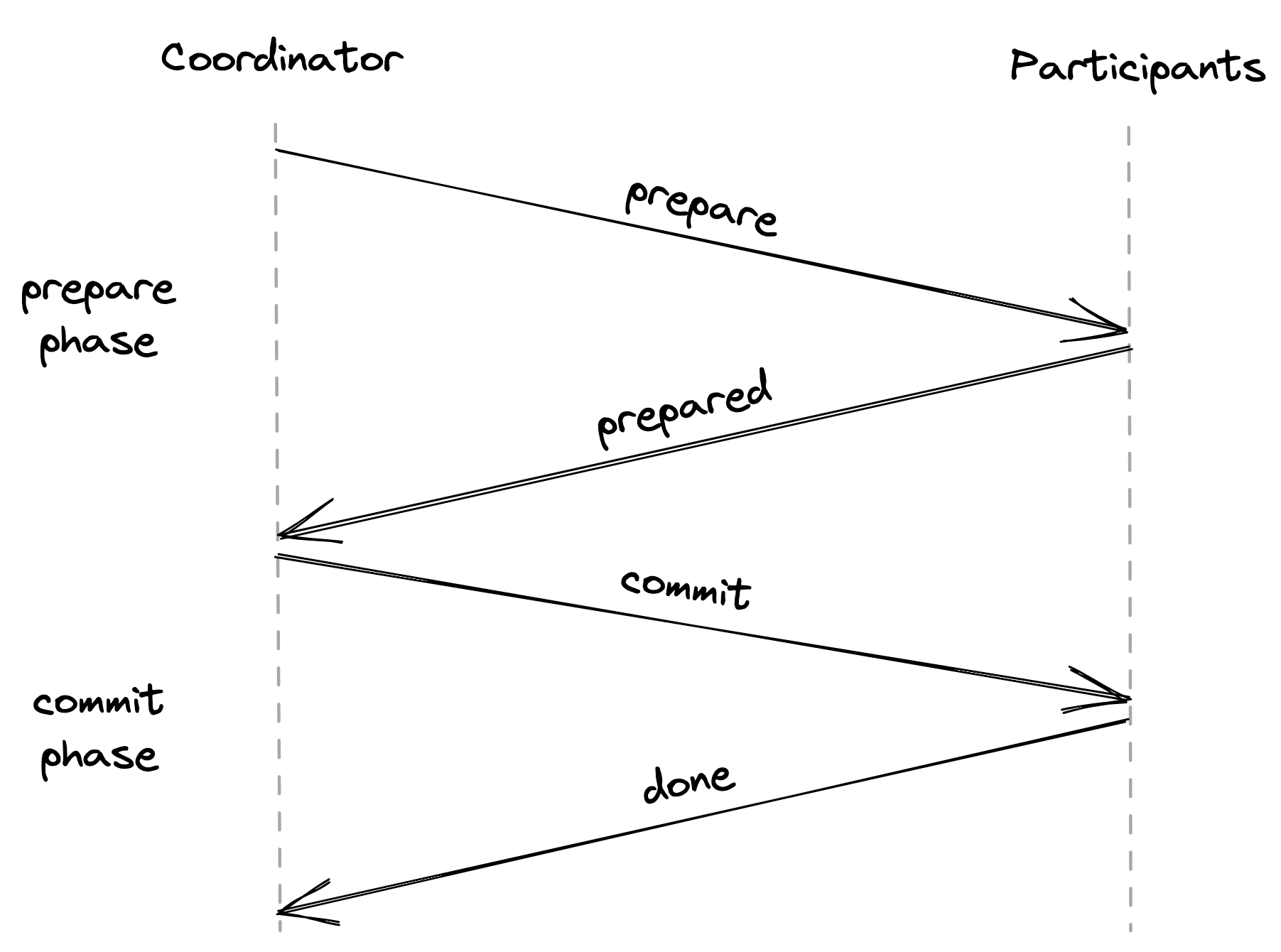
Figure 12.2: The two-phase commit protocol consists of a prepare and a commit phase.
if the coordinator crashes, the participant is stuck.
The other point of no return is when the coordinator decides to commit or abort the transaction after receiving a response to its pre-pare message from all participants. Once the coordinator makes the decision, it can’t change its mind later and has to see the transaction through to being committed or aborted, no matter what. If a participant is temporarily down, the coordinator will keep retrying until the request eventually succeeds.
Two-phase commit has a mixed reputation[14]. It’s slow since it requires multiple round trips for a transaction to complete, and if either the coordinator or a participant fails, then all processes part of the transactions are blocked until the failing process comes back online. On top of that, the participants need to implement the protocol; you can’t just take two different data stores and expect them to play ball with each other.
If we are willing to increase the complexity of the protocol, we can make it more resilient to failures by replicating the state of each process involved in the transaction. For example, replicating the coordinator with a consensus protocol like Raft makes 2PC resilient to coordinator failures. Similarly, the participants can also be replicated.
As it turns out, atomically committing a transaction is a form of consensus, called uniform consensus, where all the processes have to agree on a value, even the faulty ones. In contrast, the general form of consensus introduced in Consensus in Replication only guarantees that all non-faulty processes agree on the proposed value. Therefore, uniform consensus is actually harder[15] than consensus. Nevertheless, as mentioned earlier, general consensus can be used to replicate the state of each process and make the overall protocol more robust to failures.
NewSQL
As a historical side note, the first versions of modern large-scale data stores that came out in the late 2000s used to be referred to as NoSQL stores since their core features were focused entirely on scalability and lacked the guarantees of traditional relational databases, such as ACID transactions. But in recent years, that has started to change as distributed data stores have continued to add features that only traditional databases offered.
Arguably one of the most successful implementations of a NewSQL data store is Google’s Spanner[16]. At a high level, Spanner breaks data (key-value pairs) into partitions in order to scale. Each partition is replicated across a group of nodes in different data centers using a state machine replication protocol (Paxos).
In each replication group, there is one specific node that acts as the leader, which handles a client write transaction for that partition by first replicating it across a majority of the group and then applying it. The leader also serves as a lock manager and implements 2PL to isolate transactions modifying the partition from each other.
To support transactions that span multiple partitions, Spanner implements 2PC. A transaction is initiated by a client and coordinated by one of the group leaders of the partitions involved. All the other group leaders act as participants of the transaction (see Figure 12.3).
The coordinator logs the transaction’s state into a local write-ahead log, which is replicated across its replication group. That way, if the coordinator crashes, another node in the replication group is elected as the leader and resumes coordinating the transaction. Similarly, each participant logs the transaction’s state in its log, which is also replicated across its group. So if the participant fails, another node in the group takes over as the leader and resumes the transaction.
To guarantee isolation between transactions, Spanner uses MVCC combined with 2PL. Thanks to that, read-only transactions are lock-free and see a consistent snapshot of the data store. In contrast, write transactions use two-phase locking to create new versions of the objects they change to guarantee strict serializability.
If you recall the discussion about MVCC in Isolation in Transactions, you should know that each transaction is assigned a unique timestamp. While it’s easy to do that on a single machine, it’s a lot more challenging in a distributed setting since clocks aren’t perfectly synchronized. Although we could use a centralized timestamp service that allocates unique timestamps to transactions, it would become a scalability bottleneck. To solve this problem, Spanner uses physical clocks that, rather than returning precise timestamps, return uncertainty intervals [tearliest, tlatest] that take into account the error boundary of the measurements, where tearliest≤treal≤tlatest. So although a node doesn’t know the
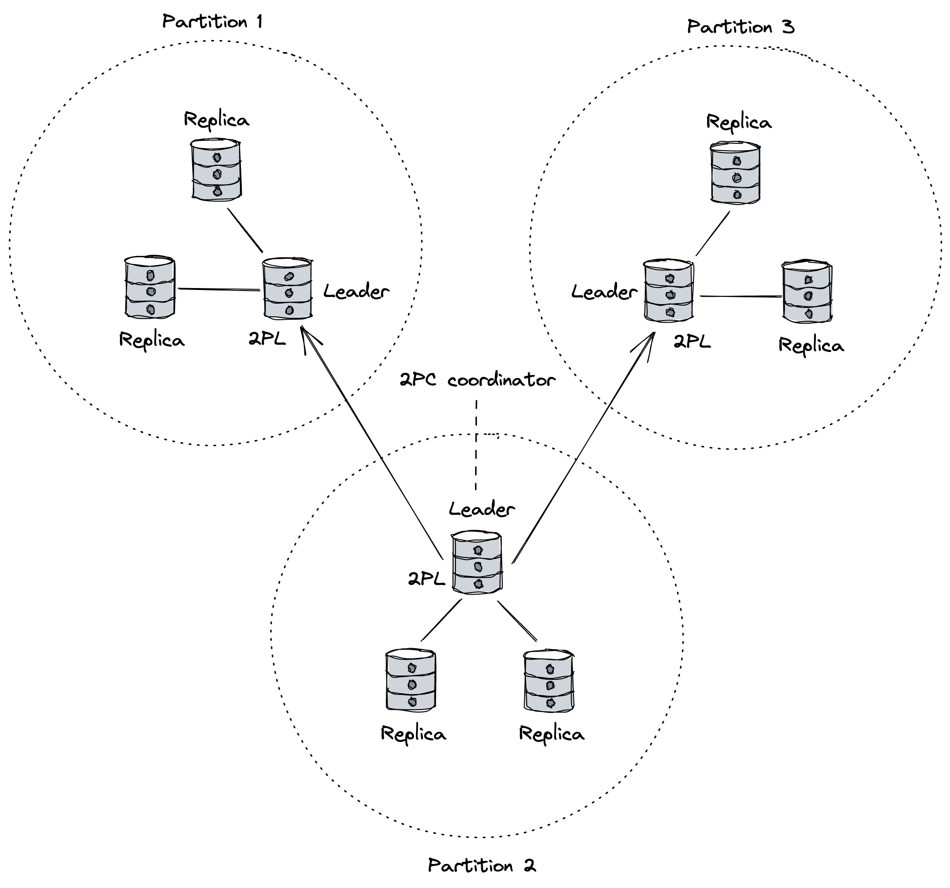
Figure 12.3: Spanner combines 2PC with 2PL and state machine replication. In this figure, there are three partitions and three replicas per partition.
current physical time treal, it knows it’s within the interval with a very high probability.
Conceptually, when a transaction wants to commit, it’s assigned the tlatesttimestamp of the interval returned by the transaction coordinator’s clock. But before the transaction can commit and release the locks, it waits for a duration equal to the uncertainty period (tlatest−tearliest). The waiting time guarantees that any transaction that starts after the previous transaction committed sees the changes applied by it. Of course, the challenge is to keep the uncertainty interval as small as possible in order for the transactions to be fast. Spanner does this by deploying GPS and atomic clocks in every data center and frequently synchronizing the quartz clocks of the nodes with them.[17]. Other systems inspired by Spanner, like CockroachDB[18], take a different approach and rely instead on hybrid-logical clocks which are composed of a physical timestamp and a logical timestamp.[19]
Asynchronous transactions
Video coming soon. Start with the reading below.
2PC is a synchronous blocking protocol — if the coordinator or any of the participants is slow or not not available, the transaction can’t make progress. Because of its blocking nature, 2PC is generally combined with a blocking concurrency control protocol, like 2PL, to provide isolation. That means the participants are holding locks while waiting for the coordinator, blocking other transactions accessing the same objects from making progress.
The underlying assumptions of 2PC are that the coordinator and the participants are available and that the duration of the transaction is short-lived. While we can do something about the participants’ availability by using state machine replication, we can’t do much about transactions that, due to their nature, take a long time to execute, like hours or days. In this case, blocking just isn’t an option. Additionally, if the participants belong to different organizations, the organizations might be unwilling to grant each other the power to block their systems to run transactions they don’t control.
To solve this problem, we can look for solutions in the real world. For example, consider a fund transfer between two banks via a cashier’s check. First, the bank issuing the check deducts the funds from the source account. Then, the check is physically transported to the other bank and there it’s finally deposited to the destination account. For the fund transfer to work, the check cannot be lost or deposited more than once. Since neither the source nor destination bank had to wait on each other while the transaction was in progress, the fund transfer via check is an asynchronous (nonblocking) atomic transaction. However, the price to pay for this is that the source and destination account are in an inconsistent state while the check is being transferred. So although asynchronous transactions are atomic, they are not isolated from each other.
Now, because a check is just a message, we can generalize this idea with the concept of persistent messages sent over the network, i.e., messages that are guaranteed to be processed exactly once. In this lesson, we will discuss a few implementations of asynchronous transactions based on this concept.
Outbox pattern
A common pattern[1] in modern applications is to replicate the same data to different data stores tailored to different use cases. For example, suppose we own a product catalog service backed by a relational database, and we decide to offer an advanced full-text search capability in its API. Although some relational databases offer a basic full-text search functionality, a dedicated service such as Elasticsearch[2] is required for more advanced use cases.
To integrate with the search service, the catalog service needs to update both the relational database and the search service when a new product is added, or an existing product is modified or deleted. The service could update the relational database first and then the search service, but if the service crashes before updating the search service, the system would be left in an inconsistent state. So we need to wrap the two updates into a transaction somehow.
We could consider using 2PC, but while the relational database supports the X/Open XA[3] 2PC standard, the search service doesn’t, which means we would have to implement the protocol for the search service somehow. We also don’t want the catalog service to block if the search service is temporarily unavailable. Although we want the two data stores to be in sync, we can accept some temporary inconsistencies. So eventual consistency is acceptable for our use case.
We can solve this problem by having the catalog service send a persistent message to the search service whenever a product is added, modified or deleted. One way of implementing that is for a local transaction to append the message to a dedicated outbox table[4] when it makes a change to the product catalog. Because the relational database supports ACID transactions, the message is appended to the outbox table if and only if the local transaction commits and is not aborted.
The outbox table can then be monitored by a dedicated relay process. When the relay process discovers a new message, it sends the message to the destination, the search service. The relay process deletes the message from the table only when it receives an acknowledgment that it was delivered successfully. Unsurprisingly, it’s possible for the same message to be delivered multiple times. For example, if the relay process crashes after sending the message but before removing it from the table, it will resend the message when it restarts. To guarantee that the destination processes the message only once, an idempotency key is assigned to it so that the message can be deduplicated (we discussed this in Idempotency in APIs).
In practice, the relay process doesn’t send messages directly to the destination. Instead, it forwards messages to a message channel[5], like Kafka[6] or Azure Event Hubs[7], responsible for delivering them to one or more destinations in the same order as they were appended. Later in Messaging (lesson 04.11), we will discuss message channels in more detail.
If you squint a little, you will see that what we have just implemented here is conceptually similar to state machine replication, where the state is represented by the products in the catalog, and the replication happens through a log of operations (the outbox table).
Sagas
Now suppose we own a travel booking service. To book a trip, the travel service has to atomically book a flight through a dedicated service and a hotel through another. However, either of these services can fail their respective request. If one booking succeeds, but the other fails, then the former needs to be canceled to guarantee atomicity. Hence, booking a trip requires multiple steps to complete, some of which are only required in case of failure. For that reason, we can’t use the simple solution presented earlier.
The Saga[8] pattern provides a solution to this problem. A saga is a distributed transaction composed of a set of local transactions T1, T2, ..., Tn, where Tihas a corresponding compensating local transaction Ciused to undo its changes. The saga guarantees that either all local transactions succeed, or, in case of failure, the compensating local transactions undo the partial execution of the transaction altogether. This guarantees the atomicity of the protocol; either all local transactions succeed, or none of them do.
Another way to think about sagas is that every local transaction Ti assumes all the other local transactions will succeed. It’s a guess, and it’s likely to be a good one, but still a guess at the end of the day. So when the guess is wrong, a mistake has been made, and an “apology[9]” needs to be issued in the form of compensating transactions Ci. This is similar to what happens in the real world when, e.g., a flight is overbooked.
A saga can be implemented with an orchestrator, i.e., the transaction coordinator, that manages the execution of the local transactions across the processes involved, i.e., the transaction’s participants. In our example, the travel booking service is the transaction’s coordinator, while the flight and hotel booking services are the transaction’s participants. The saga is composed of three local transactions: T1 books a flight, T2 books a hotel, and C1 cancels the flight booked with T1.
At a high level, the saga can be implemented with the workflow[10] depicted in Figure 13.1:
- The coordinator initiates the transaction by sending a booking request (T1) to the flight service. If the booking fails, no harm is done, and the coordinator marks the transaction as aborted.
- If the flight booking succeeds, the coordinator sends a booking request (T2) to the hotel service. If the request succeeds, the transaction is marked as successful, and we are all done.
- If the hotel booking fails, the transaction needs to be aborted. The coordinator sends a cancellation request (C1) to the flight service to cancel the previously booked flight. Without the cancellation, the transaction would be left in an inconsistent state, which would break its atomicity guarantee.
The coordinator can communicate asynchronously with the participants via message channels to tolerate temporary failures. As the transaction requires multiple steps to succeed, and the coordinator can fail at any time, it needs to persist the state of the transaction as it advances. By modeling the transaction as a state machine, the coordinator can durably checkpoint its state to a data store as it transitions from one state to the next. This ensures that if the coordinator crashes and restarts, or another process is elected as the coordinator, it can resume the transaction from where it left off by reading the last checkpoint.
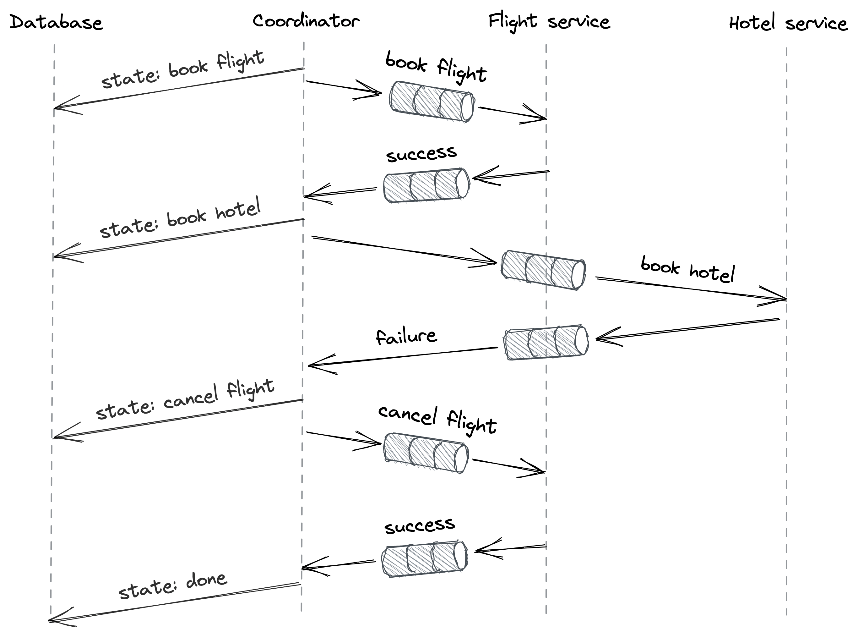
Figure 13.1: A workflow implementing an asynchronous transaction
There is a caveat, though; if the coordinator crashes after sending a request but before backing up its state, it will send the same request again when it comes back online. Similarly, if sending a request times out, the coordinator will have to retry it, causing the message to appear twice at the receiving end. Hence, the participants have to de-duplicate the messages they receive to make them idempotent.
In practice, you don’t need to build orchestration engines from scratch to implement such workflows, since cloud compute services such as AWS Step Functions[11] or Azure Durable Functions[12] make it easy to create managed workflows.
Isolation
We started our journey into asynchronous transactions as a way to work around the blocking nature of 2PC. But to do that, we had to sacrifice the isolation guarantee that traditional ACID transactions provide. As it turns out, we can work around the lack of isolation as well. For example, one way to do that is by using semantic locks[13]. The idea is that any data the saga modifies is marked with a dirty flag, which is only cleared at the end of the transaction. Another transaction trying to access a dirty record can either fail and roll back its changes or wait until the dirty flag is cleared.
If you pick any textbook about distributed systems or database systems, I guarantee you will find entire chapters dedicated to the topics discussed in this part. In fact, you can find entire books written about them! Although you could argue that it’s unlikely you will ever have to implement core distributed algorithms such as state machine replication from scratch, I feel it’s important to have seen these at least once as it will make you a better “user” of the abstractions they provide.
There are two crucial insights I would like you to take away from this part. One is that failures are unavoidable in distributed systems, and the other is that coordination is expensive.
By now, you should have realized that what makes the coordination algorithms we discussed so complex is that they must tolerate failures. Take Raft, for example. Imagine how much simpler the implementation would be if the network were reliable and processes couldn’t crash. If you were surprised by one or more edge cases in the design of Raft or chain replication, you are not alone. This stuff is hard! Fault tolerance plays a big role at any level of the stack, which is why I dedicated Resiliency (module 5) to it.
The other important takeaway is that coordination adds complexity and impacts scalability and performance. Hence, you should strive to reduce coordination when possible by:
- keeping coordination off the critical path, as chain replication does;
- proceeding without coordination and “apologize” when an inconsistency is detected, as sagas do;
- using protocols that guarantee some form of consistency without coordination, like CRDTs.
Module references
References
- “The Byzantine Generals Problem,” https://lamport.azurewebsites.net/pubs/byz.pdf
- “Unreliable Failure Detectors for Reliable Distributed Systems,” https://www.cs.utexas.edu/~lorenzo/corsi/cs380d/papers/p225-chandra.pdf
- “Introduction to Reliable and Secure Distributed Programming,” https://www.distributedprogramming.net/
- “All models are wrong,” https://en.wikipedia.org/wiki/All_models_are_wrong
References
- “Atomic clock,” https://en.wikipedia.org/wiki/Atomic_clock
- “RFC 5905: Network Time Protocol Version 4: Protocol and Algorithms Specification,” https://datatracker.ietf.org/doc/html/rfc5905
- “Time, Clocks, and the Ordering of Events in a Distributed System,” http://lamport.azurewebsites.net/pubs/time-clocks.pdf
- “Timestamps in Message-Passing Systems That Preserve the Partial Ordering,” https://fileadmin.cs.lth.se/cs/Personal/Amr_Ergawy/dist-algos-papers/4.pdf
- In actual implementations, a dictionary is used rather than an array.
- In a total order, every pair of elements is comparable. Instead, in partial order, some pairs are not comparable
- “Why Logical Clocks are Easy,” https://queue.acm.org/detail.cfm?id=2917756 6
References
- “In Search of an Understandable Consensus Algorithm,” https://raft.github.io/raft.pdf
- The same happens if the leader receives a heartbeat with a greater term.
- We will encounter one such case when discussing replication in Replication (lesson 03.06).
- We will define what linearizability means exactly later in Strong consistency in Replication.
- “Compare-and-swap,” https://en.wikipedia.org/wiki/Compare-and-swap
- “Building Distributed Locks with the DynamoDB Lock Client,” https://aws.amazon.com/blogs/database/building-distributed-locks-with-the-dynamodb-lock-client/
References
- “In Search of an Understandable Consensus Algorithm,” https://raft.github.io/raft.pdf
- “Paxos Made Simple,” https://lamport.azurewebsites.net/pubs/paxos-simple.pdf
- “Finite-state machine,” https://en.wikipedia.org/wiki/Finite-state_machine
- In practice, there are ways to reduce the number of messages required for this step.
- “Consensus,” https://en.wikipedia.org/wiki/Consensus_(computer_science)
- “Paxos made Abstract,” https://maheshba.bitbucket.io/blog/2021/11/15/Paxos.html
- We will define what linearizability means in the next section. 8nor want to, since it’s very challenging to get right; see “Paxos Made Live - An Engineering Perspective,” https://static.googleusercontent.com/media/research.google.com/en//archive/paxos_made_live.pdf
- “etcd: A distributed, reliable key-value store for the most critical data of a distributed system,” https://etcd.io/
- “Apache ZooKeeper: An open-source server which enables highly reliable distributed coordination,” https://zookeeper.apache.org/
- “Consistency Models,” https://jepsen.io/consistency
- “Linearizability,” https://jepsen.io/consistency/models/linearizable
- For example, this is the guarantee you would expect from a coordination service that manages leases.
- “Sequential Consistency,” https://jepsen.io/consistency/models/sequential
- “Perspectives on the CAP Theorem,” https://groups.csail.mit.edu/tds/papers/Gilbert/Brewer2.pdf
- “A Critique of the CAP Theorem,” https://www.cl.cam.ac.uk/research/dtg/www/files/publications/public/mk428/cap-critique.pdf
- “CAP Theorem: You don’t need CP, you don’t want AP, and you can’t have CA,” https://www.youtube.com/watch?v=hUd_9FENShA
- “Consistency Tradeoffs in Modern Distributed Database System Design,” https://en.wikipedia.org/wiki/PACELC_theorem
- “Consistency levels in Azure Cosmos DB,” https://docs.microsoft.com/en-us/azure/cosmos-db/consistency-levels
- “Apache Cassandra: How is the consistency level configured?,” https://docs.datastax.com/en/cassandra-oss/3.0/cassandra/dml/dmlConfigConsistency.html
- “Chain Replication for Supporting High Throughput and Availability,” https://www.cs.cornell.edu/home/rvr/papers/OSDI04.pdf
- This is slightly different from the original chain replication paper since it’s based on CRAQ, an extension of the original protocol; see “Object Storage on CRAQ,” https://www.usenix.org/legacy/event/usenix09/tech/full_papers/terrace/terrace.pdf .
- required for state machine replication
References
- Total order broadcast is equivalent to consensus, see “Unreliable Failure Detectors for Reliable Distributed Systems,” https://www.cs.utexas.edu/~lorenzo/corsi/cs380d/papers/p225-chandra.pdf
- “Perspectives on the CAP Theorem,” https://groups.csail.mit.edu/tds/papers/Gilbert/Brewer2.pdf
- Consensus is harder to solve than implementing a linearizable read/write register, which is what the CAP theorem uses to define consistency.
- “Gossip protocol,” https://en.wikipedia.org/wiki/Gossip_protocol
- “Strong Eventual Consistency and Conflict-free Replicated Data Types,” https://www.microsoft.com/en-us/research/video/strong-eventual-consistency-and-conflict-free-replicated-data-types/
- “Conflict-free Replicated Data Types,” https://hal.inria.fr/inria-00609399v1/document
- In practice, version vectors are used to compare the state of different replicas that only keep track of events that change the state of replicas, see “Detection of Mutual Inconsistency in Distributed Systems,” https://pages.cs.wisc.edu/~remzi/Classes/739/Fall2017/Papers/parker83detection.pdf .
- “Dynamo: Amazon’s Highly Available Key-value Store,” https://www.allthingsdistributed.com/files/amazon-dynamo-sosp2007.pdf
- “Cassandra: Open Source NoSQL Database,” https://cassandra.apache.org/
- “Riak KV: A distributed NoSQL key-value database,” https://riak.com/products/riak-kv/
- “Merkle tree,” https://en.wikipedia.org/wiki/Merkle_tree
- “Keeping CALM: When Distributed Consistency is Easy,” https://arxiv.org/pdf/1901.01930.pdf
- Consistency can have different meanings depending on the context; make sure you know precisely what it refers to when you encounter it.
- “Building on Quicksand,” https://dsf.berkeley.edu/cs286/papers/quicksand-cidr2009.pdf
- “Causal Consistency,” https://jepsen.io/consistency/models/causal
- “Consistency, Availability, and Convergence,” https://apps.cs.utexas.edu/tech_reports/reports/tr/TR-2036.pdf
- “Don’t Settle for Eventual: Scalable Causal Consistency for Wide-Area Storage with COPS,” https://www.cs.princeton.edu/~mfreed/docs/cops-sosp11.pdf
- COPS can track causal relationships between partitions (and therefore nodes), unlike simpler approaches using version vectors, which limit causality tracking to the set of keys that a single node can store (see “Session Guarantees for Weakly Consistent Replicated Data,” https://www.cs.utexas.edu/users/dahlin/Classes/GradOS/papers/SessionGuaranteesPDIS.pdf ).
- “Azure Cosmos DB: Pushing the frontier of globally distributed databases,” https://azure.microsoft.com/en-gb/blog/azure-cosmos-db-pushing-the-frontier-of-globally-distributed-databases/
References
- “Transaction processing,” https://en.wikipedia.org/wiki/Transaction_processing
- “When is”ACID” ACID? Rarely.” http://www.bailis.org/blog/when-is-acid-acid-rarely/
- see Replication (lesson 03.06)
- “PostgreSQL Transaction Isolation,” https://www.postgresql.org/docs/12/transaction-iso.html
- “Consistency Models,” https://jepsen.io/consistency
- “Jepsen Analyses,” https://jepsen.io/analyses
- “Two-phase locking,” https://en.wikipedia.org/wiki/Two-phase_locking
- “On Optimistic Methods for Concurrency Control,” https://www.eecs.harvard.edu/~htk/publication/1981-tods-kung-robinson.pdf
- “Multi-version concurrency control,” https://en.wikipedia.org/wiki/Multiversion_concurrency_control
- “CMU 15-445/645: Database Systems,” https://15445.courses.cs.cmu.edu/fall2019/
- We have already seen an example of this when discussing leases in Practical considerations in Leader election.
- The details of how this recovery mechanism works are outside the scope of this module, but you can learn more about it from any database textbook.
- “Two-phase commit protocol,” https://en.wikipedia.org/wiki/Two-phase_commit_protocol
- “It’s Time to Move on from Two Phase Commit,” http://dbmsmusings.blogspot.com/2019/01/its-time-to-move-on-from-two-phase.html
- “Uniform consensus is harder than consensus,” https://infoscience.epfl.ch/record/88273/files/CBS04.pdf?version=1
- “Spanner: Google’s Globally-Distributed Database,” https://static.googleusercontent.com/media/research.google.com/en//archive/spanner-osdi2012.pdf
- The clock uncertainty is generally less than 10ms.
- “CockroachDB,” https://www.cockroachlabs.com/
- “Logical Physical Clocks and Consistent Snapshots in Globally Distributed Databases,” https://cse.buffalo.edu/tech-reports/2014-04.pdf
References
- “Online Event Processing: Achieving consistency where distributed transactions have failed,” https://queue.acm.org/detail.cfm?id=3321612
- “Elasticsearch: A distributed, RESTful search and analytics engine,” https://www.elastic.co/elasticsearch/
- “Distributed Transaction Processing: The XA Specification,” https://pubs.opengroup.org/onlinepubs/009680699/toc.pdf
- “Pattern: Transactional outbox,” https://microservices.io/patterns/data/transactional-outbox.html
- For example, Debezium is an open source relay service that does this, see https://debezium.io/ .
- “Apache Kafka: An open-source distributed event streaming platform,” https://kafka.apache.org
- “Azure Event Hubs: A fully managed, real-time data ingestion service,” https://azure.microsoft.com/en-gb/services/event-hubs/
- “Sagas,” https://www.cs.cornell.edu/andru/cs711/2002fa/reading/sagas.pdf
- ”Building on Quicksand,” https://dsf.berkeley.edu/cs286/papers/quicksand-cidr2009.pdf
- “Clarifying the Saga pattern,” http://web.archive.org/web/20161205130022/http://kellabyte.com:80/2012/05/30/clarifying-the-saga-pattern
- “AWS Step Functions,” https://aws.amazon.com/step-functions/
- “Azure Durable Functions documentation ,” https://docs.microsoft.com/en-us/azure/azure-functions/durable/
- “Semantic ACID properties in multidatabases using remote procedure calls and update propagations,” https://dl.acm.org/doi/10.5555/284472.284478